Graph Models

In this section we’ll focus on different ways of generating graphs and the properties that arise. In particular, we will be interested in methods with properties which resemble those by social networks. Mainly, the following characteristics:

• Degree distribution: Power-law distribution.
• Avg. path length: \(O(\log N)\)
• Avg. clustering coef.: \(\simeq 10\%\)
• Existence of a giant connected component: Yes

Fixed edges model: \(G(n, m)\)

Algorithm: Start with \(n\) isolated vertices and place m edges at random between them.

Erdos-Renyi random graph: \(G(n, p)\)

Algorithm: Start with \(n\) isolated vertices and connect each pair of nodes with a probability \(p\).

Interestingly, graph properties such as diameter or probability of a giant component vs \(p\) present a threshold phenomena around \(p \simeq \frac{1}{N}\).

The characteristics achieved by this graph family:

• Degree distribution: Gaussian distribution
• Avg. path length: \(O(\log N)\)
• Avg. clustering coef: \(\simeq 0\%\)
• Existence of a giant connected component: Yes

Preferential attachment Model

Algorithm:

• Start with 2 connected nodes.

Repeat \(N-2\) times:

• Add new node \(v\)
• Create a link between \(v\) and one of the existing nodes with probability proportional to the degree

Notice there will never be triangles since we do not add links to the rest of the graph, just between the new node. The Barbasi-Albert model addresses this issue by allowing up to \(m\) connections for each added node.

• Degree distribution: Power-law distribution
• Avg. path length: \(O(\log N)\)
• Avg. clustering coef: \(\simeq 0\%\)
• Existence of a giant connected component: Yes

Configuration Model

Objective: Given a degree sequence \(k_1, ..., k_N\), build a graph with an approximate sequence:

Algorithm:

1. Assign each node a number of spokes corresponding to the degrees.
2. Randomly connect the spokes between nodes.

• Degree distribution: Any distribution! :)
• Avg. path length: \(O(\log N)\)
• Avg. clustering coef: \(\simeq 0\%\)
• Existence of a giant connected component: If the second moment minus twice the first moment of the inputed distribution is greater than zero.

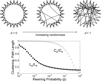
Watts-Strogatz Model (Small-World Model)

Problem: Social networks present a very high clustering coefficient and yet a very low diameter. (Small-World situations)

Algorithm:

1. Construct a regular ring lattice of \(N\) nodes connected to \(K\) neighbors.
2. For each node, with probability \(p\) re-wire a connecting edge.

Usually for \(p \simeq \frac{K}{N}\) we obtain the desired properties of:

• High clustering coefficient: Achieved by the underlying lattice structure.
• Low average path length: Achieved by the random re-wires.

Nevertheless, the degree distribution is not power law, thus resulting in unrealistic distributions.

Community-Affiliation Graph Model (AGM)

Given a set of nodes \(V\) and communities \(C\) we first assign each node to one or more communities:

Algorithm:

for each node:

• Assign one or more memberships to a given community with probability \(p_c\)

Thus, the model is uniquely defined by parameters: \(B (V, C, M, \{p_c\})\). Where \(M\) are the memberships and \(p_c\) the community probabilities. Later, we create links within the communities:

Algorithm:

for each community \(A\):

for each pair fo nodes within:

• Connect them with probability \(p_A\)

Notice that the probability of two nodes being connected is:

\begin{equation} p(u, v) = 1 - \prod_{c \in M_u \cap M_v} (1 - p_c) \end{equation}