Mining Data Streams
In this post we discuss techniques for extracting information from Data Streams. When dealing with Data Streams we make the following assumptions:
- The data arrive in one or multiple streams and must be processed immediately.
- The size of the entire stream is too big to be stored in memory or is infinite.
- The distribution of the data may be non-stationary.
There are several questions (queries) that we may want to answer by extracting information from the stream(s).
Sampling
In this section we make the assumption that data come in the form of tuples \((k, x_1, x_2, ..., x_l)\) where \(k \in K\) is a key and \(\{x_i\}\) are the attributes. One such example may be data coming from a search engine in the form (username, query, date, location, …) where username is key. Due to the assumptions above we cannot store the entire stream, but we may be interested in storing only a sample of the tuples, or a sample of tuples unfiormly distributed w.r.t. the keys.
Notation: Given a set \(S\) of tuples \(\{t_i = (k_i, x_{i, 1}, ..., x_{i, l})\}\) where \(k_i \in K\) are the keys, we define \(S^K\) as the set of unique keys in \(S\). Then, a set \(S\) is uniformly distributed w.r.t. the keys if the keys in \(S^{K}\) come from an uniform distribution in \(K\).
In order to be uniformly distributed w.r.t. the keys, the probability of \(S\) to contain a certain key must be \(1/\vert K \vert\). Therefore, the presence of a key \(k\) in \(S\) must not depend on the number of tuples that have \(k\) as key.
Sampling a fixed proportion
Assuming that we know in advance the number \(N\) of unique keys in the stream –e.g. unique users– and we want to keep a sample \(S\) containing tuples from a uniformly distributed proportion \(p=s/N\) of the keys. We can then, for each incoming tuple, hash its key with an hash function \(h: K \rightarrow \{1, ..., N\}\) and store the tuple in \(S\) if \(h(k) \le s\). If our hash function \(h\) distributes the set of keys \(K\) uniformly in \(\{1, ..., N\}\) then this method approximately keeps a proportion \(p = s/N\) of the incoming keys.
Fixed proportion sampling
Given \(N\) unique keys, \(S\) empty set, \(s\) maximum number of unique keys to store
- For each tuple \(t_n = (k_n, ...)\) in the stream
- if \(h(k_n) \le s\)
- Add \(t_n\) to \(S\)
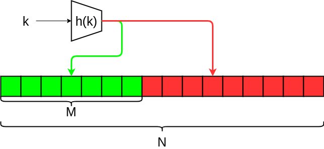
The hash function h uniformly maps keys into buckets. Tuples whose key falls in green buckets (M) are kept, others are discarded.
Sampling with fixed size
We now assume that we do not know the number of unique keys in the stream. We want to obtain a random sample \(S\) of at most \(s\) tuples uniformly distributed w.r.t. the kesy. We can use the a modified version of the Fixed proportion sampling algorithm above, by adding a threshold \(d\) that varies over time. In this case, our hash function maps keys into a very large number of buckets \(B\) and \(d\) is set to be equal to \(B\). At any time \(n\) we keep the tuple if \(h(k) \le d\). If the sample \(S\) becomes larger than \(s\), we decrease \(d\) and remove all tuples whose keys are bigger than the new value of \(d\) until the sample size is \(\le s\).
Adaptive proportion sampling
Given \(S\) empty set with maximum size \(s\), \(B\) buckets
- Set \(d=B\)
- For each tuple \(t_n = (k_n, ...)\) in the stream
- if \(h(k_n) \le d\)
- Add \(t_n\) to \(S\)
- while \(\vert S \vert > s\)
- Decrease \(d\)
- Remove all tuples \(t_j\) such that \(h(k_j) > d\)
This algorithm does not ensure, however, that the size of \(S\) is exactly \(s\) at any time, since in line 7 we remove several tuples.
The algorithm can be optimized by storing a sorted index of hash values in order to quickly remove tuples whose hash is greater than \(d\) without scanning the whole set \(S\), and \(d\) can be decreased accordingly.
If we discard the requirement of our sample being uniformly distributed w.r.t. the keys, we can obtain an algorithm that efficiently maintains a sample \(S\) of size exactly \(s\) at any time step and without the need of using an hash function. In this algorithm, called Reservoir Sampling, the set \(S\) is initially filled with the first \(s\) incoming tuples. Then, for a new tuple at time $n \gt s$, we decide to keep it with probability \(s/n\). If we keep it, we select a random tuple in \(S\) and we replace with the new one.
Reservoir sampling
Given \(S\) empty set with maximum size \(s\), \(B\) buckets
- For each tuple \(t_n = (k_n, ...)\) in the stream
- if \(\vert S\vert \lt s\)
- Add \(t_n\) to \(S\)
- else, with probability \(s/n\)
- Sample \(j \sim Uniform(1, s)\)
- \(S[j] \leftarrow t_n\)
Differently to Adaptive proportion sampling, this algorithm ensures that at each step the number of unique keys in \(S\) is exactly \(s\), at the cost of the sample not being uniform w.r.t. the keys.
The algorithm can be further improved by pre-compting the values of \(n\) at which to store the new tuple according to the Geometric distribution. This avoids us to compute a random number for each incoming tuple, and reduces the cost from \(\mathcal{O}(n)\) to \(\mathcal{O}(s(1 + \log (n/s)))\).
Filtering
A common task we may want to perform on a Data Stream is Filtering, i.e. selecting items that meet a certain criterion. Again, we assume that data come sequentially in the form of tuples $t = (k, x_1, …, x_n)$ where $k$ is the key. In the context of Data Streams, we want to perform the selection efficiently in terms of time and memory.
In particular, we are interested in the problem of membership lookup, i.e. given a set of keys \(S\), we accept a tuple \(t_i\) if \(k_i \in S\). If the set \(S\) is small enough, we can easily perform lookup by keeping \(S\) in main memory and perform quick lookup using a hash map. However, in many situations the set \(S\) does not fit in memory. In these cases, we can use a Bloom Filter to efficiently perform lookup with no false negatives and a small percentage of false positives.
Bloom Filter
A Bloom Filter is a probabilistic technique to perform hash filtering using less memory than an error-free hash lookup. Bloom Filter consists of an array \(B\) of \(N\) bits and a set \(\mathcal{H}\) of hash functions \(h_i : K \rightarrow N\) that map keys values to \(N\) buckets. First, it hashes each key in \(S\) and sets to 1 the correspondent bit in \(B\). Then, an incoming tuple is accepted only if all hash functions map it to buckets that have value 1.
Bloom Filter
Given \(S\) set of allowed keys, \(B\) array of \(N\) zeros, \(\mathcal{H} = \{h_i\}\)
- For each \(k \in S\)
- For each \(h \in \mathcal{H}\)
- \(B[h(k)] \leftarrow 1\)
- For each \(t_n\) with key \(k_n\) in the stream
- valid \(\leftarrow\) True
- For each \(h \in \mathcal{H}\)
- if \(h(k_n) = 0\) then \(valid \leftarrow False\)
- accept \(t_n\) if \(valid\)
The algorithm uses a number \(N\) of bits that is considerably smaller than that of \(S\) and ensures that there are no false negatives. The complexity of each step is \(\mathcal{O}(\vert\mathcal{H}\vert)\).
We now investigate how the probability of false positives behaves with respect to the number \(m\) of keys in \(S\), the number \(N\) of buckets, and the number \(H\) of hash functions in \(\mathcal{H}\). The probability of a key \(k \notin S\) to hash in a bit with value 1 is the probability of that bit being set to 1 in lines 1-3. We compute that probability as follows:
- For a single insertion the probability of a bit remaining 0 when hashed is \((1 - \frac{1}{N})\)
- For \(H\) hash functions, we have \((1 - \frac{1}{N})^{H}\)
- We can rewrite it as \(((1 - \frac{1}{N})^N)^{\frac{H}{N}}\)
- Remember that \(\lim_{n\rightarrow \infty} (1 - \frac{1}{n})^n = e^{-1}\)
- Then the probability of a bit to remain 0 in single insertion is \(e^{-\frac{H}{N}}\)
- For \(m\) inserted keys, the probability of the bit of still being 0 is \(e^{-\frac{mH}{N}}\)
- And the probability of the bit being 1 after \(m\) insertions is \(1 - e^{-\frac{mH}{N}}\)
Therefore, for an incoming tuple with key \(k \notin S\) the probability \(p\) of hashing to 1 for all \(h \in \mathcal{H}\) is the probability that all those buckets were set to 1 in the initialization: \begin{equation} \label{eq:p_false_pos} p(false \ positive \vert m, N, H) = \left(1 - e^{-\frac{mH}{N}}\right)^{H} \end{equation} The optimal number \(H^*\) of hash functions to use is given by \begin{equation} H^* = \frac{N}{m}\ln 2 \end{equation} and, substituting it to Eq. \ref{eq:p_false_pos} and simplifying we obtain an expression of the minimal probability of a false positive \(p*\): \begin{equation} p^* = e^{-\frac{N}{m}(\ln 2)^2} \end{equation}
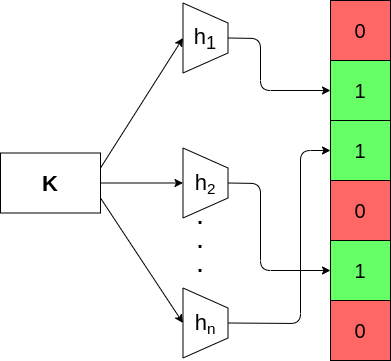
A key is mapped to buckets in the array by several hash functions.
.](/_ds/streams/bloom_ex.png)
Example of false positive probability vs number of hash functions for N = 8 billion and m = 1 billion. Picture from Mining Streams lecture of Mining of Massive Datasets.
Sliding Windows
A interesting type of queries is that of extracting information from a window of the most recent elements in the stream. Given a window of size \(N\) and enough space in memory, we can always store the whole window and be able to answer any query about it. More interesting is, however, the case in which we cannot store the whole window, due to memory constraints, or because we would not have the time to inspect all \(N\) elements at each query. For example, Amazon may be interested in knowing how many times a visit to an item led to a purchase in the last day. For each visit, we may store 1 if the item was bought and 0 otherwise. However, since the number of visits and items is huge, we need a reduced representation of the window that still allows us to approximate an answer.
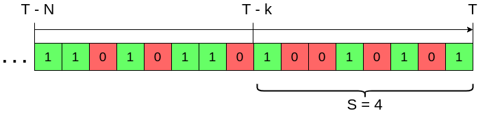
More formally, given a stream of bits \(\{b_i\}_{i=1}^{\infty}\) and being \(T\) the index of the last bit received, we want to compute \(S = \sum_{t=T-k}^T b_t\) for any value of \(k \le N\) with \(N\) being the maximum window size. In other words, we want to efficiently be able to answer thw question “How many of the last k bits were 1s?”.
DGIM Method
The DGIM Method relies on creating buckets with a fixed number of ones that grow exponentially, uses \(\mathcal{O}(\log N)\) bits and computes the number of 1s with at most 50% error, which can be reduced without changing the asymptotic memory complexity.
In DGIM, a bucket is represented by a pair \((n, t)\) where
- \(n\) is the number of ones contained in the bucket.
- \(t\) is the timestamp (modulo \(N\)) of the most recent bit in the bucket.
The algorithm works following some simple rules:
- Bucket sizes (number of ones in the bucket) must be power of 2.
- For any size \(n\), there are either 1 or 2 buckets of size \(n\)
- Buckets are non-decreasing in size as we move back in time (to the left).
- All ones belong to a bucket.
- The right end of a bucket always corresponds to a position with a 1.
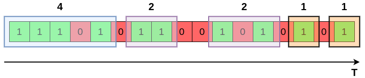
Example of DGIM bucketization. As we go back in time (left) buckets contain an increasing number of 1s that is power of 2.
Since each timestamp \(t\) is \(N\) at most, we use \(\mathcal{O}(\log N)\) bits to store it. We can store the number of ones \(n = 2^j\) by coding \(j\) in binary. Since \(j\) is at most \(\log_2 N\), we store each value \(n\) with \(\mathcal{O}(\log \log N)\) bits. The total number of buckets is \(\mathcal{O}(\log N)\) and the memory complexity of DGIM is therefore \(\mathcal{O}(\log^2 N)\).
Insertion
The algorithm is simple. When a new bit \(b\) at time \(t\) arrives, we discard it if \(b=0\). If \(b=1\), we create a new bucket with size 1 and timestamp \(t\) and we append it to the right. Then we ensure that for each size we have at most 2 buckets. If there are three buckets with size 2, we merge the two older ones into a bucket of size 4, and we repeat the process for buckets towards the left. Finally, we drop the last bucket if its timestamp goes outside the window. The DGIM insertion algorithm is therefore the following:
DGIM insert
Given \(Q = \varnothing\) queue of buckets
- For each new bit and timestamp \((b, t)\):
- if \(b = 0\)
- continue
- else
- \(t \leftarrow t \mod N\)
- \(B = (1, t)\)
- \(Q.push\_right(B)\)
- mergeBuckets(Q)
- if \(Q.peek\_left().t \le t\)
- \(Q.pop\_left()\)
where \(push\_right(B)\) appends the bucket to the right (most recent), \(peek\_left()\) inspects the left-most element (oldest) without removing it, and \(pop\_left\) removes the left-most element in the queue.
The algorithm of helper function \(mergeBuckets(Q)\) is given below. The queue is indexed left-to-right, where \(Q[0]\) is the left-most element. Each element in the queue is a bucket \(B = (n, t)\) with \(n\) the number of 1s.
mergeBuckets
Given \(Q\) queue of \(K\) buckets
- Let \(i \leftarrow K\)
- While \(i \gt 0\):
- if \(Q[i].n = Q[i - 1].n = Q[i - 2].n\)
- \(\hat{n} = Q[i-1].n + Q[i-2].n\)
- \(\hat{t} = Q[i-1].t\)
- \(\hat{B} = (\hat{n}, \hat{t})\)
- \(Q[i-2] = \hat{B}\)
- Remove \(Q[i - 1]\) and \(Q[i - 2]\) and insert \(\hat{B}\) in their place
- \(i \leftarrow i - 2\)
- else
- Return
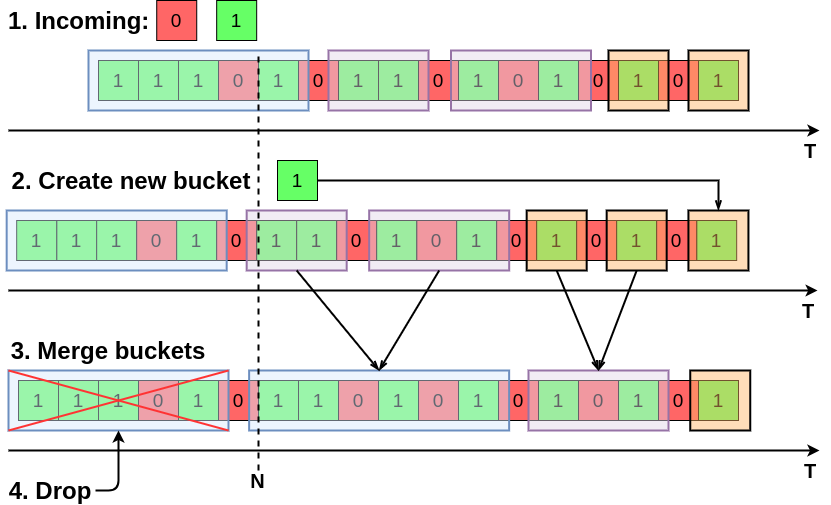
Example of DGIM insertion. Two new bits, 0 and 1, arrive. A new bucket is created for 1, leading to three buckets of size one. Then, the earliest two buckets of size one are merged into a bucket of size two, which leads to three buckets of size two. The earliest buckets of size two are merged into size four. Then, the earliest bucket is dropped as its timestamp is older than the last \(N\) elements.
We omit the check that \(i-1 \ge 0\) and \(i-2 \ge 0\) in line 3-9 for compactness. The queue may be implemented as a linked list where each element keeps a pointer to the two previous elements. This way, line 8 can be performed in \(\mathcal{O}(1)\) operations, while the memory complexity does not change asymptotically.
Note about time-stamps
To avoid the time-stamp \(t\) growing unbounded, in line 5 of DGIM we set \(t \leftarrow t \mod N\). For this reason, timestamps of buckets will not be monotonically increasing, as can be seen in the figure below. Any bit outside a window of length \(N\) will have a timestamp less or equal than the current timestamp \(t\) modulo \(N\). Therefore, the condition for dropping a bucket \(B\) is \(B.t \le (t \mod N)\), performed in line 9 of DGIM.
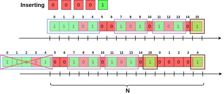
Insertion of new bits and dropping of the oldest bucket for a window \(N=16\). Time-stamp of each bit is shown. Note that the latest timestamp of the dropped bucket is equal to the timestamp of the latest bit.
Estimate the number of 1s
At any time we can estimate the number of 1s in the last \(k\) bits by inspecting buckets backwards in time (right to left). We sum the size of each bucket until we arrive at the bucket \(b\) that contains the \(k\)-th bit, and we sum half of its size to the total.
countOnes
Given \(Q\) queue of \(D\) buckets, \(k\) length of window in which to count ones, \(N\) max window size
- Let \(\hat{t} \leftarrow 0\)
- Let \(ones \leftarrow 0\)
- For \(i \leftarrow D\) down to \(2\)
- \(\Delta t \leftarrow Q[i].t - Q[i-1].t\)
- if \(\Delta t \lt 0\)
- \(\Delta t \leftarrow N + \Delta t\)
- if \(\hat{t} \lt k\)
- \(ones \leftarrow ones + Q[i].n\)
- else
- \(ones \leftarrow ones + \frac{1}{2}Q[i].n\)
- Return \(ones\)
- Return \(ones + \frac{1}{2} Q[1].n\)
If the last bucket has size \(2^r\), the maximum error we make in the estimate (line 10 or 12) is \(2^{r-1}\). Since there is at leas one bucket for each size from 0 to \(r-1\), the true sum is at least \(\sum_{i=0}^{r-1} 2^i = 2^r-1\) and the error is at most 50%.
For any bucket we only know the timestamp of its earliest 1. For this reason, we cannot know how many bits of a bucket are within the queried window of size \(k\). For this reason, we approximate their number by half the bucket size.
Lines 4-6 compute the number of bits between the latest bit of bucket \(Q[i]\) and the latest bit of bucket \(Q[i-1]\), taking into account the aforementioned considerations on the timestamp.
We can further reduce the error from 50% to \(\mathcal{O}(\frac{1}{r})\) by allowing \(r-1\) or \(r\) buckets for each size.
Counting distinct elements
In this section we discuss the problem of counting the number of distinct elements that appear in a Data Stream. For example, a website might want to count the number of unique accesses, where each access is identified by an IP number. For a popular website, storing the whole stream and count the unique IPs is unfeasible. We therefore need to fall back to techniques for, at any time, estimating the answer efficiently and using a reduced amount of memory.
The Flajolet-Martin Algorithm
The Flajolet-Martin Algorithm (or LogLog Algorithm) is an algorithm for approximating in a single pass the number of unique elements in a MultiSet, the data stream in our case. The algorithm relies on the idea that when hashing each received element, the more unique elements there are in the stream, the more different hash values we expect to see.
The hash function \(h: S \rightarrow [0, 2^L-1]\) hashes elements of the stream \(S\) into values that have binary representations of length \(L\). \(h\) is assumed to uniformly distribute its outputs, and to be deterministic (i.e. to always produce the same output for a fixed input).
Defined \(bit(x, k)\) as the \(k\)-th least significant bit of the binary representation of \(x\), such that \begin{equation} x = \sum_{k\ge 0}bit(x, k)2^k \end{equation}
We define \(\rho(x)\) as the position of the least significative 1 in the binary representation of \(x\): \begin{equation} \rho(y) = \arg\min_{k} {bit(x, k)} \end{equation}
For example, \(8 = 1000_2\) then \(\rho(8) = 3\) since the first bit set to 1 in the binary representation is at position 3.
and we set \(\rho(0) = L\).
Reaing values from the stream with the Flajolet-Martin Algorithm is very simple:
flajoletMartinInsert
Given \(S\) the stream, \(h\) the hash function with \(L\) length of binary representation
- Let \(V\) be an array of \(L\) 0s
- For each \(x \in S\)
- \(i = \rho(h(x))\)
- \(V[i] = 1\)
And, to compute the number of unique elements, we use the \(flajoletMartinCount\) procedure:
flajoletMartinCount
Given \(V\) the bit array, \(\phi = 0.77351\)
- Let \(R \leftarrow \arg\min_{i} V[i] = 0\)
- Return \(2^R / \phi\)
where \(\phi\) is a correction factor (see the paper for details). The amount of memory used by the algorithm is therefore \(L\) bits. The complexity of each insertion is given by only computing the hash function and can be considered \(\mathcal{O}(1)\). The complexity of counting is \(\mathcal{O}(L)\).
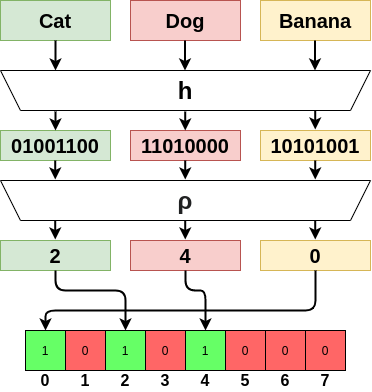
Example of reading elements from stream in the Flajolet-Martin algorithm.
To see why it works, we observe that:
- The probability that a given \(h(a)\) ends in at least \(r\) trailing zeros is \(2^{-r}\).
- Then, the probability of not seeing a tail of length \(r\) after reading \(m\) elements is \((1 - 2^{-r})^m\)
- The latter can be written as \((1 - 2^{-r})^{2^r(m2^{-r})} \approx e^{-\frac{m}{2^r}}\)
- If \(m \ll 2^r\) then \(e^{-\frac{m}{2^r}} \rightarrow 1\)
- If \(m \gg 2^r\) then \(e^{-\frac{m}{2^r}} \rightarrow 0\).
- Then, \(2^r\) will almost always be around to \(m\).
The Flajolet-Martin algorithm, however, presents some issues. The expected value of the solution \(\mathbb{E}[2^R]\) is infinite, since when the probability of \(R\) trailing zeros halves, the value doubles. The solution has high variance, and for every bit “off” the value \(2^R\) doubles. A way to mitigate this behavior is to use several hash functions and compute the mean or the median of the estimated values.
HyperLogLog
Published in 2007 by Flajolet et al., HyperLogLog is an extension to the Flajolet-Martin algorithm to address the problem of high variance. The algorithm works by splitting the stream into \(2^b\) streams and computing the armonic mean of their estimated cardinality. The HyperLogLog algorithm keeps \(2^b\) registers of \(L\) bits. When an element \(x\) arrives, \(h(x)\vert_1^b\) (the first \(b\) bits of \(h(x)\)) are used to select a register. The value of the register is then set as the maximum between the current value and \(\rho(h(x)\vert_{b+1}^{L})\)
hyperloglogAdd
Given \(M\) a memory of \(m=2^b\) registers, \(h\) hash function
- For each element \(e\) in the stream
- \(x = h(e)\)
- \(i = x\vert_1^b\)
- \(M[i] = \max(M[i], \rho(x\vert_{b+1}^L))\)
The count is then performed by computing \begin{equation} Z = \Big(\sum_{j=1}^{m}2^{-M[j]}\Big)^{-1} \end{equation}
\begin{equation} \alpha_m = \Big(m \int_0^{\infty} \Big(\log_2\Big(\frac{2+u}{1+u}\Big)\Big)^{m}du\Big)^{-1} \end{equation}
\begin{equation} count = \alpha_m m^2 Z \end{equation}
The HyperLogLog paper gives a formal explanation of the algorithm. Less formally, if \(n\) is the unknown cardinality of the stream \(S\), then in each of the \(m\) register will end up \(n/m\) elements. Thus, \(\max_{x \in M[j]} \rho(x)\) should be close to \(\log_2 (n/m)\) and the armonic mean is \(mZ\). Therefore, \(m^2Z\) should be approximately \(n\). The term \(\alpha_m\) corrects for the multiplicative bias in \(m^2Z\).