Until now we had to manually design the reward function. IRL automatically learns the reward function from expert demonstrations. In this case, instead of hard-coding a reward we would provide demonstrations.
This is different from imitation learning (IL) since IL does not reason about the outcome of actions, it just tries to mimic the demonstrations.
Problem: Learning the reward is an underspecified problem, multiple reward functions may explain the same expert behavior.
Feature matching IRL
We can model the reward function with any approximator (linear, GP, ANNs…), if using linear:
\begin{equation} r_\psi (s, a) = \sum_i \psi_i f_i (s, a) = \psi^T f(s, a) \end{equation}
Where \(f\) are the state-action features. In this case, if \(\pi^{r_\psi}\) is the optimal policy for \(r_\psi\), we want to pick \(\psi\) such that the expectations of features our own and the expert policies match (thus the name of feature matching):
\begin{equation} E_{\pi^{r_\psi}} [f(s, a)] = E_{\pi^*} [f(s, a)] \end{equation}
We can estimate the RHS by:
\(E_{\pi^*} [f(s, a)] = \sum_{(s, a)} f(s, a) \cdot prop((s, a))\)
for all \((s, a)\) observed.
Where \(prop((s, a))\) is the proportion of times the pair \((s, a)\) appears in the dataset.
For the LHS, if the env. dynamics are unknown we can produce samples and do the same (very costly but works).
Otherwise, for known small env. dynamics we could apply dynamic programming to learn it.
To find the optimal parameters we can get inspiration from SVM optimization and use hte maximum margin principle: Maximize the parameters \(\psi\) which provide a larger margin \(m\) between
\begin{equation} max_{\psi, m} m \space \space \space s.t. \psi^T E_{\pi^\star} [f(s, a)] \geq max_{\pi \in \Pi} \psi^T E_{\pi} [f(s, a)] + m \end{equation}
Where we can apply the SVM trick, and instead of using a margin of 1, use some distance between policies so that we do not force a margin on very similar policies:
\begin{equation} max_{\psi} \frac{1}{2} \Vert \psi \Vert^2 \space \space \space s.t. \psi^T E_{\pi^*} [f(s, a)] \geq max_{\pi \in \Pi} \psi^T E_{\pi} [f(s, a)] + D ( \pi, \pi^\star ) \end{equation}
Problems:
- Maximizing the margin is a bit arbitrary
- What if the “expert” demonstrations are suboptimal? We could add slack variables as in a SVM setup.
- It might be ok for this linear case but become very messy for ANN reward approximation.
Maximum Entropy IRL (MaxEntr IRL)
This framework accounts for the uncertainty in the demonstrators examples.
Learning the optimality variable \(r\) in small spaces
As we saw in Lecture 14: Control as Inference, we can design probabilistic models to describe near-optimal behavior.
We can infer the optimality by seeing how probable a trajectory is.
In this section we’ll apply same idea to learn the reward function instead: \(r_\psi (s, a)\), where \(\psi\) are the parameters which describe \(r\).
Remember that:
\begin{equation} p(O_t \mid s_t, a_t, \psi) = exp \left( r_\psi (s_t, a_t) \right) \end{equation}
\begin{equation} p(\tau \mid O_{1:T}, \psi) \propto p(\tau) exp \left( \sum_t r_\psi (s_t, a_t) \right) \end{equation}
Therefore, if we apply maximum likelihood learning, we need to maximize:
\begin{equation} max_\psi \frac{1}{N} \sum_i \log p(\tau_i \mid O_{1:T}, \psi) \end{equation}
Where if we ignore the transition probabilities (since they are independent from \(\psi\)):
\begin{equation} max_\psi \frac{1}{N} \sum_i r_\psi ( \tau_i ) - \log (Z) \end{equation}
Where \(Z\) is the partition function (makes the computation way harder):
\begin{equation} Z = \int p(\tau) exp(r_\psi (\tau)) d \tau \end{equation}
Which can be interpreted as “make the reward on the seen trajectories (expert demonstrations) big w.r.t the other possible trajectories that the expert did not execute”.\
Substituting and taking derivatives:
\begin{equation} \nabla_\psi \mathcal{L} = \frac{1}{N} \sum_i \nabla_\psi r_\psi (\tau_i) - \frac{1}{Z} \int p(\tau) exp(r_\psi(\tau)) \nabla_\psi r_\psi(\tau) d \tau \end{equation}
Which can be nicely re-written as:
\begin{equation} \label{grad} \nabla_\psi \mathcal{L} = E_{\tau \sim \pi^\star (\tau)} \left[ \nabla_\psi r_\psi (\tau_i) \right] - E_{\tau \sim p(\tau \mid O_{1:T}, \psi)} \left[ \nabla_\psi r_\psi(\tau) \right] \end{equation}
The gradient of the likelihood points into the positive direction for the trajectories that come from the expert. And negative direction for the samples of the policy corresponding to the current reward. Cancelling to zero when both distributions are equal.
Computing the first expectation is easy using the experts samples, so now we’ll focus on computing the soft optimal policy under current reward.
Estimating the expectation (second term in eq. \ref{grad}):
Using the linearity of the expectation:
\begin{equation} E_{\tau \sim p(\tau \mid O_{1:T}, \psi)} \left[ \nabla_\psi r_\psi(\tau) \right] = \sum_t E_{(s_t, a_t) \sim p(s_t, a_t \mid O_{1:T}, \psi)} \left[ \nabla_\psi r_\psi(s_t, a_t) \right] \end{equation}
Where if we break \(p(s_t, a_t \mid O_{1:T}, \psi) = p(a_t \mid O_{1:T}, \psi) p(s_t \mid O_{1:T}, \psi)\), which as we saw in Lecture 14: Control as Inference, \(p(a_t \mid O_{1:T}, \psi) p(s_t \mid O_{1:T}, \psi) \propto \beta(s_t, a_t) \alpha(s_t)\) where \(\beta\) is the backward message, and \(\alpha\) the forward message.
This requires the state-action space to be small enough so you can go through every single state and action (still much better than working with trajectories, which grow exponentially with the number of states-actions). This is instead linear in time-horizon, state, and action space.
Defining \(\mu_t(s_t, a_t) \propto \beta(s_t, a_t) \alpha(s_t)\) (normalized) we get:
\begin{equation} E_{\tau \sim p(\tau \mid O_{1:T}, \psi)} \left[ \nabla_\psi r_\psi(\tau) \right] = \sum_t \int \int \mu_t(s_t, a_t) \nabla_\psi r_\psi(\tau) ds_t da_t = \sum_t \vec{\mu_t}^T \cdot \vec{r}_\psi \end{equation}
\(\vec{\mu_t}\) is the state-action visitation probability for each \((s_t, a_t)\).
With this, we can finally define the MaxEnt IRL algorithm ():
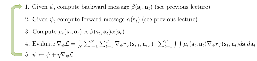
MaxEntr IRL algorithm
This works well for small (tabular) state-action spaces with known transitions.
This framework is called max-entropy because it can be shown in the case where: \(r_\psi (s_t, a_t) = \psi^T f(s_t, a_t)\), it optimizes: \(max_\psi \mathcal{H} \left( \pi^{r_\psi} \right) \space \space s.t. E_{\pi^{r_\psi}}[f] = E_{\pi^\star} [f]\). Which is like saying “get the most random policy which matches the expert”. It is good because it doesn’t do any more assumptions on the behavior other than this one.
Learning the optimality variable \(r\) in big spaces
So far MaxEnt IRL required:
- Solving for soft optimal policy in the inner loop
- Enumerating all state-action tuples (to get visitation frequency and gradient).
For practical problems we need:
- Large and continuous spaces
- States obtained via sampling only
- Unknown dynamics
Unknown dynamics & large state-action spaces
Under the assumption we do not know the dynamics but we can sample from the env., we can use any maximum-entropy RL algorithm seen in previous lectures to learn \(p(a_t \mid s_t, O_{1:T}, \psi)\).
Which could be done as :
\begin{equation} \nabla_\psi \mathcal{L} \simeq \frac{1}{N} \sum_i \nabla_\psi r_\psi (\tau_i) - \frac{1}{M} \sum_j \nabla_\psi r_\psi (\tau_j) \end{equation}
Where the first term are expert demonstrations and the second one policy samples.
Problem: We need to make the learning of \(p(a_t \mid s_t, O_{1:T}, \psi)\) converge for every step of the \(\psi\) optimization \(\Rightarrow\) Very slow!
Solution: Instead of re-learning a policy after each step of \(\psi\) optimization, we can have a single one and do single steps to optimize it. For instance, we can use importance sampling:
\begin{equation} \nabla_\psi \mathcal{L} \simeq \frac{1}{N} \sum_i \nabla_\psi r_\psi (\tau_i) - \frac{1}{\sum_j w_j} \sum_j w_j \nabla_\psi r_\psi (\tau_j) \end{equation}
Where: \(w_j = \frac{p(\tau) exp ( r_\psi (\tau_j) ) }{\pi(\tau_j)}\), which if we expand using trajectory probabilities a lot gets cancelled out: \(w_j = \frac{exp \left( \sum_t r_\psi (s_t, a_t)\right)}{\prod_t \pi (a_t \mid s_t)}\).
This lazy update of the policy samples w.r.t \(r_\psi\) brings us closer to the target distribution!
Guided cost learning algorithm exemplifies how to use this approach:
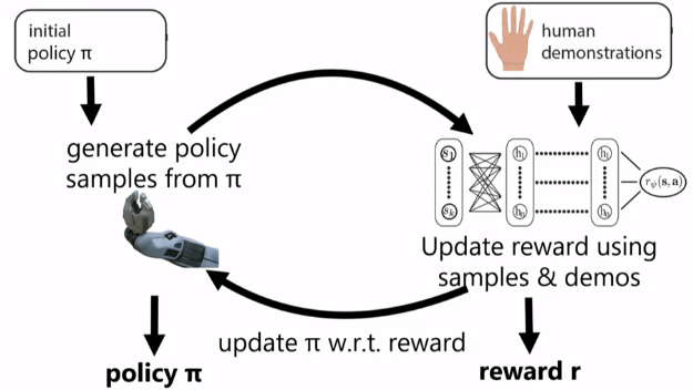
Guided cost learning algorithm
Reward and policy are sort of “competing” against each other: Policy demos are made less likely by the reward optimization, and then the policy optimization adapts to the new reward to create better policies in an iterative manner. Once everything converges the policy is indistinct from the demonstration policy. This idea is very similar to the one of Generative Adversarial Networks (GANs). Where the generator can be seen as our policy and the discriminator as our reward function.
More on this connection between GANs and IRL in this paper.
Another GAN IRL algorithm in this paper.
Yet another which even takes the similarities in a more direct way: paper.