At this point you might be wondering something like: Wait, if we have demonstrations on how to behave in an environment, can’t we just fit a model capable of generalizing (e.g. ANN) to it? That is what Imitation Learning tries to achieve, sadly it doesn’t work. In this post we explain why.
Behavioral Cloning (BC)
IDEA: Record a lot of “expert” demonstrations and apply classic supervised learning to obtain a model to map observations to actions (policy).
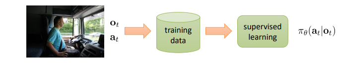
Self-driving vehicle behavioral cloning workflow example. We can safe a dataset of expert observation-action pairs and train a ANN to learn the mapping from observation to action.
Behavioral cloning is a type of Imitation Learning -a general term to say “learn from expert demonstrations”.
Behavioral cloning is just a fancy way to say “supervised learning”.
Why doesn’t this work?
1. Distributional shift
Wrong actions change the data distribution: A small mistake makes the subsequent observation distribution to be different from the training data. This makes the policy to be more prone to error: it has not been trained on this new distribution (as the expert did not commit mistakes). This snowball effect keeps rising the error between trajectories over time:
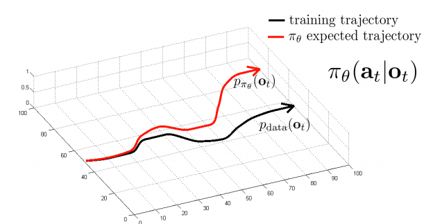
Representation of the distributional shift problem.
Improvements:
- Using some application-specific “hacks”: Self-driving car and Drone trained with BC.
- Adding noise to training trajectory so its more robust against errors.
- Adding a penalty for deviating (inverse RL idea)
- DAgger algorithm (Dataset Aggregation)
DAgger algorithm
Idea: Collect training data from policy distribution instead of human distribution, using the following algorithm:
- Train \(\pi_{\theta} (a_t \mid o_t)\) on expert data: \(\mathcal{D} = (o_1, a_1, ..., o_N, a_N)\)
- Run \(\pi_{\theta} (a_t \mid o_t)\) to get a dataset \(\mathcal{D}_\pi = (o_1, ..., o_N)\).
- Ask expert to label \(\mathcal{D}_\pi\) with actions \(a_t\).
- Aggregate \(\mathcal{D} \leftarrow \mathcal{D} \cup \mathcal{D}_\pi\)
- Repeat
Problem: While it addresses the distributional shift problem, it is and unnatural way for humans to provide labels (we expect temporal coherence) \(\Rightarrow\) Bad labels.
2. Non-Markovian behavior
Most decision humans take are non-Markovian: If we see the same thing twice we won’t act exactly the same (given only the last time-step). What happened in previous time-steps affects our current actions. This makes the training much harder.
Improvements:
- We could feed the whole history to the model but the input would be too large to train robustly.
- We can use a RNN approach to account for the time dependency.
Problems:
- Causal Confusion: Training models with history may exacerbate wrong causal relationships.
3. Multimodal behavior
In a continuous action space, if the parametric distribution chosen for our policy is not multimodal (e.g. a single Gaussian) the Maximum Likelihood Estimation (MLE) of the actions may be a problem:
While both ‘go left’ and ‘go right’ actions are ok, the average action is bad.
Improvements:
- Output a mixture of Gaussians: \(\pi (a \mid o) = \sum_i w_i \mathcal{N} (\mu_i, \Sigma_i)\)
- Latent variable models: Can be as expressive as we want: We can feed to the network a prior variable sampled from a known distribution. In this case, the policy training is harder but can be done using a technique like:
- Conditional variational autoencoder
- Normalizing flow/realNVP
- Stein variational gradient descent
- Autoregressive discretization: Convert the continuous action space into a discrete one using neural nets. The idea is to sequentially discretize one dimension at a time:
- Feed-forward policy network to obtain each action continuous distribution.
- Split first dimension into bins and sample as a categorical distribution.
- Feed-forward this sampled value into a new small NN with inputs the \(n-1\) other actions and outputs the \(n-1\) other actions again.
- Repeat from 2. until all actions are discretized.
Quantitative analysis
Defining the cost function: \(c(s, a) = \delta_{a \neq \pi^*(s)}\) (1 when the action is different from the expert).
And assuming that the probability of making a mistake on a state sampled from the training distribution is bounded by \(\epsilon\): \(\space \space \pi_\theta (a \neq \pi^* (s) \mid s) \leq \epsilon \space\space \forall s \sim p_{train}(s)\)
Case \(p_{train}(s) \simeq p_{\theta}(s)\):
\begin{equation} E \left[ \sum_t c(s_t, a_t) \right] = O(\epsilon T) \end{equation}
This would be the case if DAgger algorithm correctly applied, where the training data distribution converges to the trained policy one.
Case \(p_{train}(s) \neq p_{\theta}(s)\):
We have that: \(p_\theta (s_t) = (1-\epsilon)^t p_{train} (s_t) + (1 - (1 - \epsilon)^t) p_{mistake} (s_t)\)
Where \(p_{mistake} (s_t)\) is a state probability distribution different from \(p_{train} (s_t)\). In the worst case, the total variation divergence: \(\mid p_{mistake} (s_t) - p_{train} (s_t) \mid = 2\)
Therefore:
\begin{equation} \sum_t E_{p_\theta (s_t)} [c_t] = O(\epsilon T^2) \end{equation}
The error expectation grows quadratically over time!! More details on: A Reduction of Imitation Learning and Structured Prediction to No-Regret Online Learning