In this lecture we focus on the case where we have an explicit, differentiable policy that maps a given state to the correspondent distribution over actions. In deep RL this is tipically achieved by a Neural Network, but other function approximation techniques may be used.
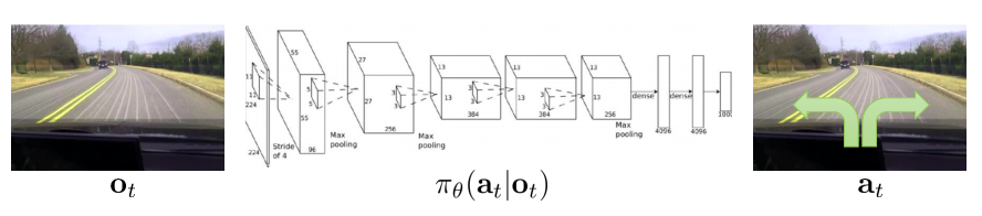
Example of a policy modeled by a Convolutional Neural NetworkExample of a policy modeled by a Convolutional Neural Network
Notation
Such a policy is parametrized by a set of parameters \(\theta\) that can be, for example, the weights of a Neural Network. Thus, \(\pi_{\theta}(a | s)\) represents the probability of chosing action \(a\) given the current state \(s\). We use \(\pi_{\theta}(\tau)\) to represent the probability of a trajectory $\tau$. We represent the total reward of a trajectory \(\tau\) as \(r(\tau)\).
Direct Policy Differentiation
We aim to maximize the objective function \(J(\theta)\) of Eq. \ref{eq:objective}. We can do this by exploiting the common gradient step technique. \begin{equation} \label{eq:objective} J(\theta) = E_{\tau \sim \pi_{\theta}(\tau)}[r(\tau)] \end{equation}
Exploiting the log gradient trick we obtain that \begin{equation} \label{eq:objective_gradient} \nabla_{\theta} J(\theta) = E_{\tau \sim \pi_{\theta}(\tau)}[ \nabla_{\theta}\log \pi_{\theta}(\tau) r(\tau)] \end{equation}
Then, by plugging in \(\pi_{\theta}(\tau) = p(s_1) \prod_{t=1}^T \pi_{\theta}(a_t \vert s_t) p(s_{t+1} \vert s_t, a_t)\) into the log in Eq.\ref{eq:objective_gradient} and observing that the gradient is zero for all the terms not depending on \(\theta\), we obtain
\begin{equation} \label{eq:policy_gradient} \nabla_{\theta}J(\theta) = E_{\tau \sim \pi_{\theta}(\tau)} \left [\left (\sum_{t=1}^T \nabla_{\theta}\log \pi_{\theta}(a_t \vert s_t) \right ) r(\tau) \right] \end{equation}
A more detailed explanation of the steps that bring to this result can be found in the Annex 5: Policy Gradients. We are now left with the problem of computing this gradient, that is defined as an expectation over the trajectory distribution. Since we assume to not know the dynamics of the environment, we cannot directly compute this distribution and its expected value. Instead, we use Monte Carlo sampling to obtain an unbiased estimate of the gradient. We sample \(N\) trajectories \(\tau^{(i)}\), \(i = 1\) … \(N\), by running the policy in the environment, and we compute the gradient \(\nabla_{\theta}J(\theta)\)
\begin{equation} \label{eq:gradient_sample} \nabla_{\theta}J(\theta) = \frac{1}{N} \sum_{i=1}^N \left(\sum_{t=1}^T \nabla_{\theta}\log \pi_{\theta}(a_t^{(i)} \vert s_t^{(i)}) \right) r(\tau^{(i)}) \end{equation}
where \(r(\tau^{(i)})\) is the total reward of the \(i\)-th trajectory.
REINFORCE
We now have everything we need to introduce the basic REINFORCE algorithm.
- Initialize \(\theta\) at random
- While not converged
- Run policy \(\pi_{\theta}\) in the environment and collect trajectories \(\{\tau^{(i)}\}\)
- Compute \(\nabla_{\theta}J(\theta) \approx \sum_{i=1}^N \left( \sum_{t=1}^T \nabla_{\theta}\log \pi_{\theta}(a_t^{(i)} \vert s_t^{(i)}) \right) r(\tau^{(i)})\)
- \[\theta = \theta + \alpha \nabla_{\theta}J(\theta)\]
The equation of the gradient does not contain the term \(\frac{1}{N}\) because the magnitude of the gradient is already determined by the learning rate \(\alpha\).
Interpretation
We now reason about what does Eq. \ref{eq:policy_gradient} do. When we take a gradient step given by \(E_{\tau \sim \pi_{\theta}(\tau)} [\nabla_{\theta}\log \pi_{\theta}(\tau)]\) we are making the trajectory \(\tau\) more probale. If we multiply the term inside the gradient by \(r(\tau)\) as in Eq. \ref{eq:policy_gradient}, we increase/decrease the likelihood of the trajectory in consideration depending on the sign of \(r(\tau)\). Thus, if the total reward \(r(\tau)\) is negative, the likelihood of the trajectory \(\tau\) is decreased, while if it is positive it is increased. Increasing or decreasing the likelihood of a trajectory \(\tau\) means that the gradient step is increasing/decreasing the likelihood of the actions \(a_t\) correspondent to the states \(s_t\) for \(a_t, s_t \in \tau\). This, however, poses some serious issues that in practice make the Policy Gradient technique as we stated it not working.
How to make Policy Gradient work
As formulated above, the Policy Gradient methods do not really work well. In this section we analyze their main issues and the tricks necessary to make Policy Gradient algorithms work.
The causality issue
The term \(r(\tau)\) in Eq.\ref{eq:gradient_sample} is the total reward of a trajectory \(\tau\): \begin{equation} r(\tau) = \sum_{t=1}^T r(s_t, a_t) \end{equation} with \(s_t\), \(a_t\) being the state and action at time-step \(t\) in the trajectory \(\tau\). If we develop Eq. \ref{eq:policy_gradient} by expliciting \(r(\tau)\) and moving it inside the summation we obtain
\begin{equation} \nabla_{\theta}J(\theta) = E_{\tau \sim \pi_{\theta}(\tau)} \left [\sum_{t=1}^T \left ( \nabla_{\theta}\log \pi_{\theta}(a_t \vert s_t) \sum_{t=1}^T r(s_t, a_t) \right ) \right] \end{equation}
We can observe that each gradient term \(\nabla_{\theta}\log \pi_{\theta}(a_t \vert s_t)\) is multiplied by the sum of rewards \(r(\tau) = \sum_{t=1}^T r(s_t, a_t)\), which is the total reward of the trajectory, starting from the first step. Therefore, the gradient of the policy at \(a_t\) and \(s_t\) is influenced also by the rewards obtained before the time-step \(t\). This inevitably leads to a confusion in the algorithm, that can increase the likelihood of bad actions thanks to rewards obtained before that action was taken -i.e. the causality is not taken into consideration.
This can be solved by using the so called reward to go \(\hat{Q}_t = \sum_{t'=t}^T r(s_t, a_t)\) that is the total reward of a trajectory \(\tau\) from the time-step \(t\) onwards. Eq. \ref{eq:policy_gradient} then becomes
\begin{equation} \label{eq:pg_togo} \nabla_{\theta}J(\theta) = E_{\tau \sim \pi_{\theta}(\tau)} \left [\sum_{t=1}^T \nabla_{\theta}\log \pi_{\theta}(a_t \vert s_t) \hat{Q}_t \right] \end{equation}
Baselines
In the interpretation we said that the gradient steps increases the likelihood of trajectories with positive rewards and decreases the likelihood of those with negative rewards. Consider the case in which we have some trajectories with positive rewards, and some with negative rewards (in green in the figure). The action distribution is correctly pushed towards the trajectories with positive rewards. However, if we add an offset to the same rewards making them all positive without changing their scale (yellow in the figure), things change dramatically. Now, the gradient step is correctly pushing the action distribution towards the higher rewards, but it is also spreading it in the direction of the lower -but still positive- ones, since the gradient step is also increasing their likelihood.
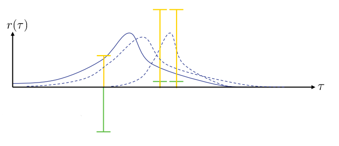
Example of rewards with same relative scale but different offsets.
A solution to this issue is to use a baseline. As we explain more in detail in the Annex 5: Policy Gradients, we can subtract any term $b$ that does not depend on the trajectory \(\tau\) from Eq. \ref{eq:gradient_sample}, obtaining \begin{equation} \nabla_{\theta}J(\theta) = \frac{1}{N} \sum_{i=1}^N \sum_{t=1}^T \nabla_{\theta}\log \pi_{\theta}(a_t^{(i)} \vert s_t^{(i)}) \left( r(\tau^{(i)}) - b \right) \end{equation}
where \(b\) is the mean reward over the sampled trajectories \begin{equation} b = \frac{1}{N} \sum_{i=1}^N r(\tau^{(i)}) \end{equation}
Off-Policy Policy Gradient
The Policy Gradient we analyzed in on-policy: since expectations are taken over the distribution \(\pi_{\theta}\), every time we update \(\theta\) with the gradient step, we need to collect more samples of experience. This is not an issue if the samples are generated by a cheap simulator, but can become a real problem when generating samples of experience is costly. We therefore need to be able to reuse past experience.
It is possible to compute expectations over a distribution \(p(x)\) by using samples obtained from another distribution \(q(x)\) by exploiting importance sampling, where \begin{equation} E_{x \sim p(x)}[f(x)] = E_{x \sim q(x)}\left[\frac{p(x)}{q(x)}f(x)\right] \end{equation}
This is exactly what we need, since we want to compute the gradient of Eq. \ref{eq:policy_gradient} for the new policy \(\pi_{\theta'}\) by exploiting samples obtained under the old policy \(\pi_{\theta}\). The objective function now becomes \begin{equation} J(\theta) = E_{\tau \sim \pi_{\theta}(\tau)} \left [ \frac{\pi_{\theta’}(\tau)}{\pi_{\theta}(\tau)} r(\tau) \right ] \end{equation}
and we observe that the state transition probabilities cancel out in the ratio \begin{equation} \frac{\pi_{\theta’}(\tau)}{\pi_{\theta}(\tau)} = \frac{p(s_1) \prod_{t=1}^T \pi_{\theta’}(a_t \vert s_t) p(s_{t+1} \vert s_t, a_t)} {p(s_1) \prod_{t=1}^T \pi_{\theta}(a_t \vert s_t) p(s_{t+1} \vert s_t, a_t)} = \prod_{t=1}^T \frac{\pi_{\theta’}(a_t \vert s_t)} {\pi_{\theta}(a_t \vert s_t)} \end{equation}
obtaining the gradient for off-policy Policy Gradient
\begin{equation} \nabla_{\theta’}J(\theta’) = E_{\tau \sim \pi_{\theta}(\tau)} \left [ \left ( \prod_{t=1}^T \frac{\pi_{\theta’}(a_t \vert s_t)}{\pi_{\theta}(a_t \vert s_t)} \right ) \left ( \sum_{t=1}^T \nabla_{\theta’} \log \pi_{\theta’}(a_t \vert s_t) \right) r(\tau) \right ] \end{equation}
we can employ the causality fix that we described above by using the reward to go and by doing the same for the importance weights
\begin{equation} \label{eq:off_policy} \nabla_{\theta’}J(\theta’) = E_{\tau \sim \pi_{\theta}} \left [ \sum_{t=1}^T \nabla_{\theta’}\log \pi_{\theta’}(a_t \vert s_t) \left( \prod_{t’=1}^t \frac{\pi_{\theta’}(a_{t’}\vert s_{t’})}{\pi_{\theta}(a_{t’} \vert s_{t’})} \right) \left( \sum_{t’=t}^T r(s_{t’}, a_{t’}) \prod_{t^{\prime\prime}=t}^{t’} \frac{\pi_{\theta’}(a_{t^{\prime\prime}}\vert s_{t^{\prime\prime}})} {\pi_{\theta}(a_{t^{\prime\prime}} \vert s_{t^{\prime\prime}})} \right) \right ] \end{equation}
If we try to implement this function, we will likely incur into underflow issues, due to the multiplication of many small numbers together. We can remove second product of importance weights (the right-most one). This simplifies the equation and, for reasons that will be explained later in the lectures, still leaves us with a gradient that improves the policy.

However, the issue remains with the left-most product of importance weights. We resort to a first order approximation by substituting the product of the importance weights with the correspondent state-action marginal distributions \(\pi_{\theta'}(s_t, a_t)\) and \(\pi_{\theta}(s_t, a_t)\). We can factorize them by applying the chain rule \(\pi(s_t, a_t) = \pi(s_t) \pi(a_t \vert s_t)\) where the term \(\pi(s_t)\) is the state marginal distribution that we do not know. However, it can be shown that we can remove this term as long as the new policy \(\theta'\) is close enough to the old \(\theta\). The resulting off-policy Policy Gradient will then be
\begin{equation} \label{eq:off_policy_approx} \nabla_{\theta’}J(\theta’) = \frac{1}{N} \sum_{i=1}^N \sum_{t=1}^T \frac{\pi_{\theta’}(a_t^{(i)} \vert s_t^{(i)})}{\pi_{\theta}(a_t^{(i)} \vert s_t^{(i)})} \nabla_{\theta’}\log\pi_{\theta’}(a_t^{(i)} \vert s_t^{(i)}) \hat{Q}_{i, t} \end{equation} in which we used the reward to go \(\hat{Q}_{i, t}\), i.e. the total reward of the \(i\)-th trajectory from time-step \(t\) onwards.
Which off-policy setting should I implement?
The goal of off-policy algorithms is to reuse experience collected with elder versions of the policy as much as possible. The formulation of Eq. \ref{eq:off_policy} allows us to use samples obtained from any distribution \(\pi_{\theta}\), but has the issue that for big values of \(T\) it can lead to numerical instabilities. On the other hand, the formulation of Eq. \ref{eq:off_policy_approx} requires the old policy \(\pi_{\theta}\) to be close enough to the new policy \(\pi_{\theta'}\), preventing us to exploit samples from policies that are too different, but solves the numerical issues. Therefore, if the time horizon \(T\) is not too big, the formulation of Eq. \ref{eq:off_policy} is preferrable, otherwise one should go for Eq. \ref{eq:off_policy_approx}.