In this lecture we go over again the two algorithms we studied in Lecture 7: Value Function Methods, Fitted Q iteration and Q Learning, we point out their main issues and discuss how to actually make them work with Neural Networks. Then, we discuss how to make Q Learning work in a continuous actions setting.
Q Learning Issues
The Q-Learning algorithm we previously described is the following
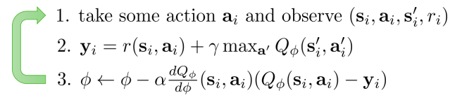
Q Learning algorithm
which is an online version of the Fitted Q Iteration algorithm
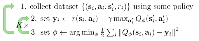
Fitted Q Iteration
There is a fundamental difference between the Q Learning and the Fitted Q Iteration algorithms. While in Q-Learning we learn while the agent collects experience, in Fitted Q Iteration we collect the whole experience dataset first, and then we perform a full regression on it. Then, we use the learned policy to collect a new dataset, and we repeat. This is however not optimal for large networks, as it becomes too expensive to train on the whole dataset at each iteration.
Q-Learning is NOT gradient descent
The step 3 of Q-Learning looks very similar to the Gradient Descent algorithm, which we know converges. But looking more closely, the targets \(\pmb{y}_i\) depend on the parameters \(\phi\) in step 2, but no gradient flows trough them. Therefore, we are not guaranteed that this gradient updates will converge to anything useful.
One-step gradient
\(Q_{\phi}\) is a Neural Network, and we know that it is hard to train Neural Networks with gradient from a single sample -this is why we use batches. This issue is not present in the Fitted Q Iteration algorithm, that collects a batch of transitions before performing the gradient update, but it is a problem if we try to use the online version, Q-Learning.
Moving targets
In Q-Learning, after each gradient step the targets are computed from the network we just updated. Each gradient step is therefore updating the network towards a target that is constantly changing, preventing the process to converge. This does not happen in Fitted Q Iteration, as steps 2 and 3 perform a supervised regression on fixed targets.
Correlated samples
Both Q-Learning and Fitted Q Iteration suffer from the fact that the collected samples are correlated, since they come from the agent interacting with the environment and, therefore, subsequent states will have high correlation and will be similar. Each gradient update will therefore overfit to the current neighborhood of states and forget what it learned before.
Solving the issues
We now explain some solutions to the issues above and derive an algorithm that puts all the fixes together
Replay Buffers
Since these algorithms are off-policy, we do not need to use the latest collected transitions to perform the gradient step. We can instead store a dataset of transitions, coming from one or multiple parallel workers, and sample from this dataset batches of transitions from which we compute the targets and perform the gradient step.
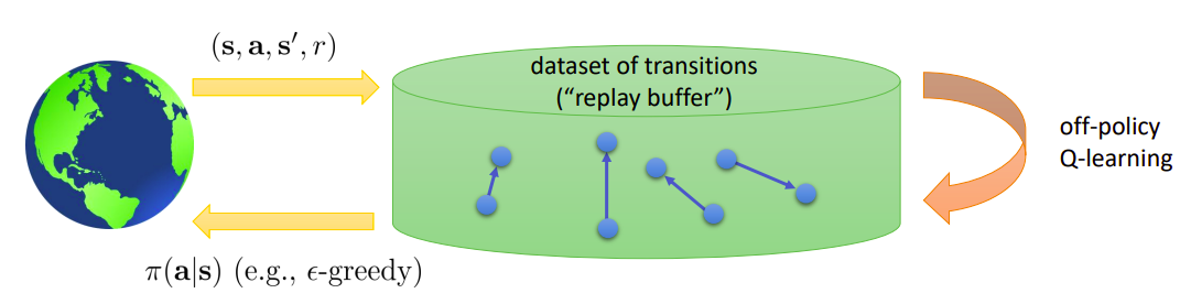
A replay buffer acts as a dataset of transitions. It is filled by interacting with the environment, but the learning is off-policy
We now have to decide how often to refill the replay buffer, how many transitions to store, and how to sample transitions for the off-policy learning. Replay buffers solve the one-step gradient issue, as well as the correlated samples issues.
Target Networks
We are left with one issue that is present in Q-Learning but not in Fitted Q Iteration: the moving targets. We saw that Fitted Q Iteration does not have this issue, since it performs a well-defined regression. We want to achieve the same result, i.e. a stable regression on fixed targets, but bringing it into a more online algorithm. A good way of obtaining this is using a fixed version of a recent \(Q_{\phi}\) network when computing the targets. This way, targets will remain stable while the learning network \(Q_{\phi}\) is trained. Then, we update the target network parameters \(\phi'\) with the trained parameters \(\phi\), and repeat the process.
Deep Q Learning
We now have everything we need to define a class of deep Q-Learning algorithms that actually work, by adding a replay buffer and a target network.

These algorithms work alternating between the following steps in different ways:
- Data collection: we store transitions in a replay buffer by running an exploration policy in the environment.
- Target update: we update the target network with the trained network. We can do this every \(N\) steps or at each step by performing a slight update \(\phi' \leftarrow \tau\phi' + (1 - \tau)\phi\).
- Q function regression: we train the learning network \(Q_{\phi}\) from the targets computed by the target network \(Q_{\phi'}\) for \(K\) gradient updates.
By varying how often these 3 operations are carried out, we can derive different algorithms of this class. The general algorithm is the following

In the well-known DQN algorithm, (Mnih et al, 2013), the first to successfully play Atari games directly from visual inputs, we have \(N=1\) and \(K=1\).
Double Q-Learning
The Q-Learning framework suffers from an overestimation issue. The target values are computed from \begin{equation} \label{eq:targets} y = r + \gamma \max_{a’}Q_{\phi’}(s’, a’) \end{equation}
It can be shown that, for \(n\) random variables \(X_1\), .. \(X_n\), \begin{equation} E\left[\max(X_1,\ …,\ X_n)\right] \ge max(E[X_1],\ …,\ E[X_n]) \end{equation} Therefore, when we perform the \(\max\) operation in the targets of Eq. \ref{eq:targets}, we are systematically overestimating the Q values. Since taking the \(\max\) over the \(Q_{\phi'}\) values is equivalent to taking the \(Q_{\phi'}\) value of the \(\arg\max\) action \begin{equation} \label{eq:max_q} \max_{a’}Q_{\phi’}(s’, a’) = Q_{\phi}(s’, \arg\max_{a’}Q_{\phi’}(s’, a’)) \end{equation} both the selected action (in the \(\arg\max\) ) and the value of that action are taken from the same network \(Q_{\phi'}\): the same noise affects both.
In order to decorrelate this error, we will use two networks, one for choosing the action, and the other to compute its value. Luckily, we already have two networks, the learning and the target network. In Double Q Learning, we compute the targets of Eq. \ref{eq:targets} as
\begin{equation} y = r + \gamma Q_{\phi’}(s’, \arg\max_{a’}Q_{\phi}(s’, a’)) \end{equation}
Note how the action is chosen according to an \(\arg\max\) over \(Q_{\phi}\), while its value is computed with \(Q_{\phi'}\).
Multi Step Returns
The targets computed by Eq. \ref{eq:targets} are composed of a single reward term and a bootstrapped estimate of the total return from that state onwards, the \(Q\) term. The \(Q\) term dominates the sum, as it represent the total discounted reward. If the \(Q\) term is inaccurate, we are in troulbe, as the targets we are learning from are dominated by it. We are therefore tempted to use multi-step returns, as we did in Policy Gradient or Actor-Critics. We can therefore compute the targets as \begin{equation} y_t = \sum_{t’=t}^{t+N-1} \gamma^{t’-t} r_{t’} + \gamma^{N} \max_{a}Q_{\phi}(s_{t+N}, a) \end{equation} in which the parameter \(N\) trades off between lower variance but high biased targets (low \(N\)) and high variance but low biased targets (high \(N\)).
This however has a troublesome consequence: the algorithm is now correct only when learning on-policy. In fact, the sum of \(N\) rewards now corresponds to a particular trajectory obtained by the policy under which they were collected and therefore represent an estimate of the cumulative reward for the current policy \(\pi\). There are a few ways of solving this issue:
- Ignore the problem: often works well, roughly for \(N \le 4\)
- Cut the trace: cut the rewards sequence at \(K \le N\) such that the \(K\) actions taken in the sequence are the same that would have been taken by the current policy
- Importance sampling: see Munos et al., 2016
Q Learning with Continuous Actions
When dealing with continuous actions we have some troubles in computing targets of Eq. \ref{eq:targets}. While for discrete actions we can easiy compute the Q value for each of the possible actions and take the bigger, we cannot do the same when actions are continuous. Here we show a brief analysis of some techniques for dealing with continuous actions.
Stochastic Optimization
A very simple and efficient solution is to sample \(N\) actions \(a_1\), …, \(a_N\) from the action space and chose the one that has the highest Q value: \begin{equation} \max_a Q_{\phi}(s, a) \approx max(Q_{\phi}(s, a_1),\ …,\ Q_{\phi}(s, a_N)) \end{equation} This technique is not really accurate, but is really fast and the maximization can be efficiently parallelized, thus lot of samples can be evaluated.
More accurate solutions are:
- Cross Entropy Methods: sample \(N\) actions, fit a proposed distribution by minimizing the cross-entropy, and repeat. This leads to increasingly better samples that maximize the Q value.
- CMA-ES: an evolutionay strategies method
Easily Maximizable Q Functions
If our task has a complex state space but roughly simple actions, we can design a Q function in which the output is a complex combination of the state but a combination of the action of which computing the one that maximizes the Q value is straight-forward.
In the NAF architecture (Normalized Advantage Functions) the Q values are given by a combination of the Neural Network outputs that is quadratic in the action: \begin{equation} \label{eq:max} Q_{\phi}(s, a) = -\frac{1}{2}(a - \mu_{\phi}(s))^T P_{\phi}(s)(a - \mu_{\phi}(s)) + V_{\phi}(s) \end{equation}
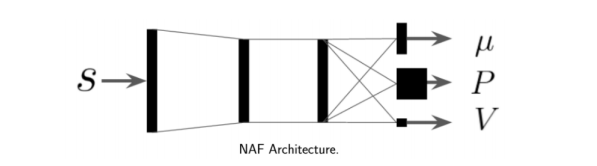
Since only the quadratic term depends on the action, and the maximum of the given quadratic form is \(\mu_{\phi}(s)\), we obtain \begin{equation} \arg\max_a Q_{\phi}(s, a) = \mu_{\phi}(s) \end{equation} and \begin{equation} \max_a Q_{\phi}(s, a) = V_{\phi}(s) \end{equation}
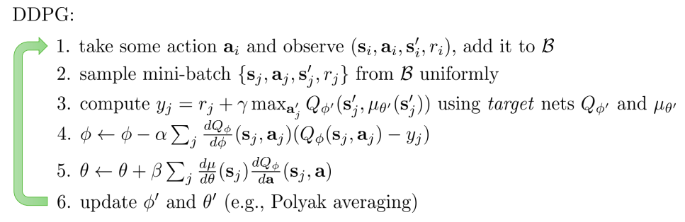
DDPG (Deep Deterministic Policy Gradient)
Another option to perform the \(\max\) operation is to exploit the formulation of Eq. \ref{eq:max} and train another network \(\mu_{\theta}(s)\) to approximate the \(\arg\max_a Q_{\phi}(s, a)\). We therefore need to find \(\theta\) such that:
\begin{equation} \theta \leftarrow \arg\max_{\theta} Q_{\phi}(s, \mu_{\theta}(s)) \end{equation}
This can be done by exploiting the chain rule to compute \begin{equation} \frac{dQ_{\phi}}{d\theta} = \frac{da}{d\theta} \frac{dQ_{\phi}}{da} \end{equation}
We obtain the DDPG algorithm:
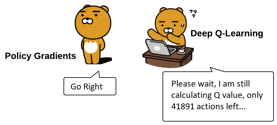
PG vs DQN:
At this point we can understand this meme: