Probability Distributions
This post is more a memory-refresher list of the most famous probability distributions rather than a comprehensive explanation of anything in particular.
Discrete
Bernoulli
Toss of a coin with probability of head of \(\lambda \in [0, 1]\).
\begin{equation} X \in \{0, 1\} \end{equation}
\begin{equation} p(X = x \mid \lambda) = \begin{cases} \lambda & \textrm{if} \space x = 1 \newline 1-\lambda & \textrm{if} \space x = 0 \end{cases} \end{equation}
Moments Example: By means of example, its moments would be computed as:
\[E [X] = \sum_x p(x) x = \lambda \cdot 1 + (1 - \lambda) \cdot 0 = \lambda\]\(V [X] = E [(X - E (X))^2] = E [(X - \lambda)^2] = p(0) (0 - \lambda)^2 + p(1) (1 - \lambda)^2 = \lambda (1 - \lambda)\)
Categorical
Toss of a dice with \(k\) faces and probabilities \(\lambda_1, ..., \lambda_k\). Where \(\sum_i \lambda_i = 1\), and \(\lambda_i \in [0, 1] \forall i\).
\begin{equation} X \in \{1:k\} \end{equation}
\begin{equation} p(X=x \mid \lambda_{i=1:N}) = \begin{cases} \lambda_1 & \textrm{if} \space x = 1 \newline \lambda_2 & \textrm{if} \space x = 2 \newline … \end{cases} \end{equation}
Remember: Categorical Cross-Entropy is often used as a loss function for ML supervised classification tasks, which is:
\[\mathcal{H} (P, Q) = E_P [I_Q] = - \sum_{i} p(P=p_i) \log (Q = p_i) = - \sum \lambda_i \log (\hat \lambda_i)\]In classification tasks, we see our model prediction as a categorical distribution: for a given input, a certain probability is assigned to each class. In this context:
\(P\) is the “real” categorical distribution of the data. Usually the labels come as a 1-hot encoding: so the “real” distribution we want to match has probability \(1\) in the correct label and \(0\) in the others. \(\hat \lambda_i\) indicates whether class \(i\) is the correct one for a given input.
\(Q\) on the other hand, is the guess done by our model, with each \(\lambda_i\) being the probability of classifying the input into class \(i\).
Thus, the loss associated with a datapoint becomes: \(- \log (\hat \lambda_i)\) (negative log of the guessed prob).
Remember that the cross-entropy is often used when the data information is fixed, thus the KL divergence: \(D_{KL} (P \Vert Q) = E_P [I_Q - I_P] = \mathcal{H} (P, Q) + \underbrace{\mathcal{H} (P)}_{const}\).
Binomial
Number of successes in \(n\) Bernoullies (with mean \(\lambda \in [0, 1]\)).
\begin{equation} X \in \{1:n\} \end{equation}
\begin{equation} p(X = x \mid \lambda) = {N \choose x} \lambda^x (1 - \lambda)^{n - x} \end{equation}
For large \(n\) and \(\lambda \simeq \frac{1}{2}\) it behaves as a discretization of the Gaussian distribution.
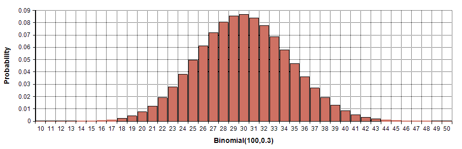
Binomial PMF
Multinomial
Number of counts of a k-sided die rolled n times. I.e. \(x_i\) counts the number of times side \(i\) appeared when rolling the dice \(n\) times, thus:
\begin{equation} x_{i \in 1:k} \in \{0:n\} \end{equation}
Where: \(\sum_{i=1}^k x_i = n\)
\begin{equation} p(X=\{x_1, …, x_k\} \mid N, \lambda_{i=1:N}) = {N \choose {x_1, …, x_k}} \lambda_1^{x_1} … \lambda_k^{x_k} \end{equation}
Notice this is a generalization of binomial distribution for categorical variables: Instead of counting successes of a bernoulli event, we count successes of a categorical event.
Geometric
Counts the number of failures before the first success in a Bernoulli r.v.
\begin{equation} x \in \mathbb{N} \end{equation}
\begin{equation} p(X = x \mid \lambda) = (1 - \lambda)^{x-1} \lambda \end{equation}
Usage example: This distribution is often used to model life expectancy of something that has a probability \(\lambda\) of dying at every time-step. For instance, in RL: if life expectancy of an agent is \(E[X] = \frac{1}{\lambda}\), we discount each expected future reward by a factor of \(\lambda\) to account for the probability of being alive at that point (there are other reasons to discount it such as making infinite episode reward sums finite or account for the fact that most actions do not have long-lasting repercussions).
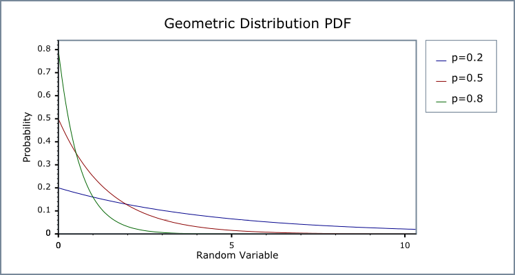
Geometric PMF
Poisson
Counts the number of random independent events happening in a fixed period of time (or space):
Imagine that on average \(\lambda \in \mathbb{R}_{> 0}\) events happen within a time period (aka Poison process). We can then get the probability of \(x\) events happening in this time-period using the Poisson distribution:
\begin{equation} x \in \mathbb{N} \end{equation}
\begin{equation} p(X = x \mid \lambda) = \frac{\lambda^x e^{- \lambda}}{x!} \end{equation}
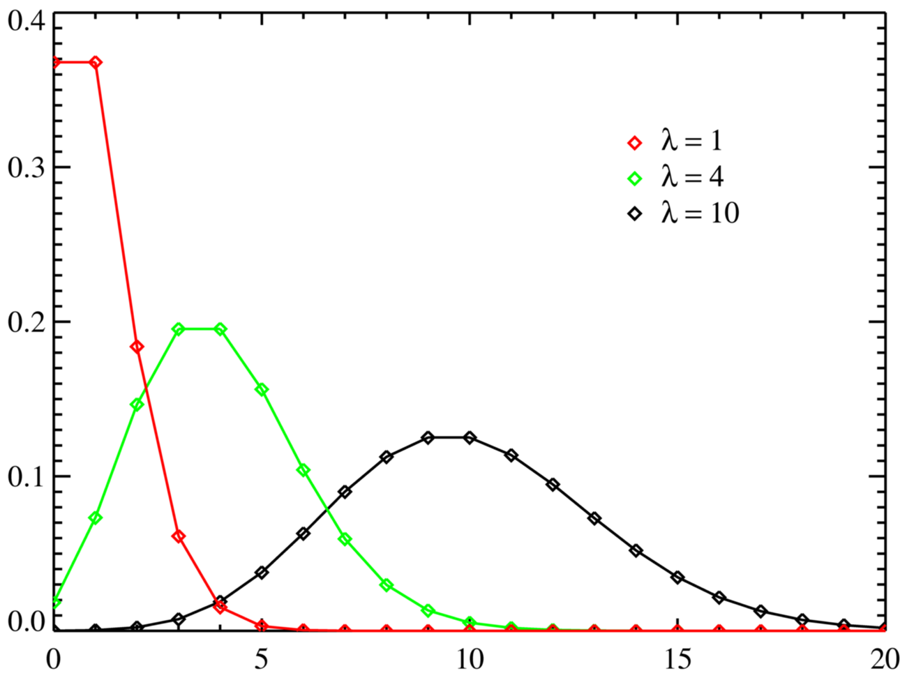
Poisson PMF
Continuous
Uniform
Assigns same likelihood to all values between a range.
\begin{equation} x \in [a, b] \end{equation}
\begin{equation} PDF(x, a, b) = \frac{1}{b-a} \end{equation}
- Is the distribution which gives the maximum entropy for \(x \in [a, b]\)
MLE Example: By means of example, lets see how we would compute the MLE of its parameters given a dataset \(\mathcal{D} = \\{ x_i \\}_{i=1:n}\). If we express the likelihood of the dataset we get that:
\begin{equation} \mathcal{L (\mathcal{D}, a, b)} = \left(\frac{1}{b - a} \right)^n \end{equation}
If we want to maximize the likelihood, we need to minimize \(b - a\) but \(x_i \in [a, b] \forall i\). Thus, the minimum is achieved when:
\begin{equation} a = \min_i x_i \space \space b = \max_i x_i \end{equation}
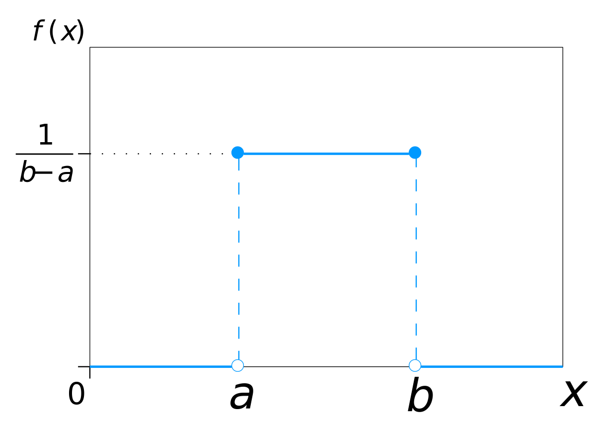
Uniform PDF
Gaussian/Normal
\begin{equation} x \in \mathbb{R} \end{equation}
\begin{equation} PDF(x, \mu, \sigma) = \frac{1}{\sqrt{2 \pi \sigma^2}} e^{- \frac{1}{2} \frac{(x - \mu)^2}{\sigma^2}} \end{equation}
- Is the distribution which gives the maximum entropy for a fixed \(\mu, \sigma^2\) for \(x \in \mathbb{R}\).
- A property which makes the Gaussian distribution extremely analytically tractable is its closure under linear combinations: The linear combination of Gaussian r.v.’s is Gaussian.
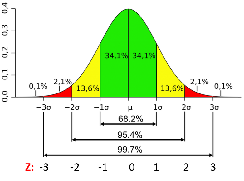
Gaussian PDF
Weak Law of Large Numbers
The mean of a sequence of i.i.d random variables converges in probability to the expected value of the random variable as the length of that sequence tends to infinity:
\begin{equation} \bar X_n \overset{p}{\to} E[X] \end{equation}
Converges in probability means that the probability of the sample’s mean being equal to the distribution mean tends to 0 as the sample size grows: \(\lim_{n \rightarrow \infty} p(\vert \bar X_n - E[X] \vert > \epsilon) = 0 \space \space \forall \epsilon \in \mathbb{R}_{>0}\)
This is very nice, but it only considers the mean of a SINGLE set of samples of a random variable. But what distribution does this mean follow?
Central limit theorem
The distribution of sample means of any distribution converges in distribution to a normal distribution.
\begin{equation} \frac{\bar{X}_n - \mu}{\sigma\sqrt{n}} \xrightarrow{d} N(0,1), \end{equation}
This only applies to finite-mean and finite-variance distributions, so forget about stuff like Cauchy distribution.
Converges in distribution means that the CDF of the set of means converges to the CDF of a Gaussian distribution.
Combining these two theorems, we can assume that the mean of samples of any distribution will follow a normal distribution around the expected value if the sample size is big enough (usually 30 samples is considered big enough).
The central limit theorem gives the impression that a lot of events in nature seem to follow a normal distribution. Thus, it is very often the case that scientists assume normality on their observations (also because of the maximum entropy principle)
Chi-squared \(\chi^2\)
Models the sum of k squared standardized normals.
\begin{equation} x \in (0, \infty) \end{equation}
\begin{equation} PDF(x, k) = \frac{1}{\Gamma (k) 2^{\frac{k}{2}}} x^{\frac{k}{2} - 1} e^{- \frac{x}{2}} \end{equation}
Exponential
Represents the distribution probability of the amount of time between two Poison-type events. Measures the amount of time probability between two Poisson-type events. \(\lambda\) again is the expected number of events within the time period.
\begin{equation} x \in [0, \infty) \end{equation}
\begin{equation} PDF(x, \lambda) = \lambda e^{- \lambda x} \end{equation}
It is often said that “it doesn’t have memory, this happens because the occurrence of events are independent from each other. The way I picture it is with this process:
- Throw \(\lambda\) darts into a 1-dimensional target of fixed length
- Walk through the target from side to side.
The probability distribution of time to the next dart is exponential and it doesn’t matter that you just saw one, the probability of seeing another one is completely unrelated:
\begin{equation} p(x > s + t \mid x > s) = p(x > t) \end{equation}
Can be thought of as a continuous version of a Geometric distribution. “Number of failures until one success” is analogous to “time until event”.
Gamma
The same way the exponential distribution predicts the amount of time until the first Poisson event, the Gamma distribution predicts the time until the k-th Poisson of event having rate \(\lambda \frac{\text{events}}{\text{timeperiod}}\).
\begin{equation} x \in (0, \infty) \end{equation}
Presents two representations. One with shape parameter \(k\) (“number” of events) and scale parameters \(\theta = \frac{1}{\lambda}\) (inverse of Poisson rate \(\lambda\)):
\begin{equation} PDF(x, k, \theta) = \frac{1}{\Gamma (\alpha) \theta^k} x^{k - 1} e^{- \frac{x}{\theta}} \end{equation}
And one with shape (\(\alpha = k\) “number” of events) and rate parameters \(\beta = \frac{1}{\theta}\). Notice that this rate is the same as the dictated by the Poisson distribution: \(\beta = \lambda\))
\begin{equation} PDF(x, \alpha, \beta) = \frac{\beta^\alpha}{\Gamma (\alpha)} x^{\alpha - 1} e^{- \beta x} \end{equation}
- It is the distribution which gives a maximum entropy for a fixed \(E[X] = k \theta = \frac{\alpha}{\beta} \geq 0\) for \(x \in (0, \infty)\)
- Exponential (k=1), \(\chi^2\), and Erlang distributions are particular cases of Gamma distribution.
- It is often used as a conjugate prior of other distributions.
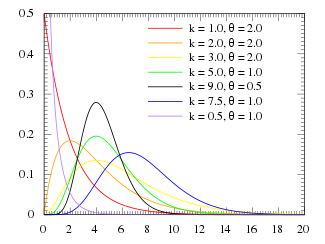
Gamma PDF