Grad-CAM: Visual Explanations from Deep Networks via Gradient-based Localization
IDEA
ANNs lack of decomposability into independent components makes it very challenging to understand their “reasoning”. Visual explanations (VE) can help with this issue in every state of AI development. Compared to humans, when AI is:
- Weaker: VE are useful to detect failure models.
- On pair: VE are useful to establish trust to their users. (e.g. Image recognition with enough data)
- Stronger: VE are useful to explain to humans. Known as machine teaching. (e.g. Chess or GO)
This paper develops on this challenge with 2 contributions:
- Generalizes the Class Activation Mapping (CAM) method for detecting attention areas. They call this algorithm Grad-CAM.
- It combines the previous algorithm with Guided BackPropagation to detect the key features of the relevant area. They call this algorithm Guided Grad-CAM.
Consider a CNN-based image classification task. Given an input image and a label, CAM provides a heatmap over the image of the area which is more relevant for that particular label. Nevertheless its applicability is quite limited. It only supports fully CNN models, i.e. models which do not have any non-convolutional layer. This paper presents a more general approach which works on any architecture whose first model is a CNN.
Consider the following architecture:
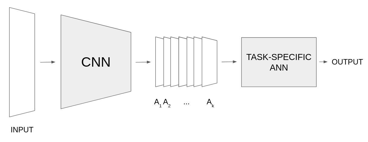
Figure 1: Grad-CAM supported architecure. Input image gets converted to a k-channel feature map, which later is processed by any ANN. (Figure from CampusAI)
The task-specific ANN varies depending on the application. For instance, it can be a combination of Dense layers for image classification or a RNN for image captioning or question answering.
Grad-CAM
Given an input image and a label \(y^c\), Grad-CAM provides a heatmap of the areas of the image which are relevant to the model for that given label. The algorithm goes as follows:
- Feed-forward the input image through the CNN model and get the feature-map: \(A_1, ..., A_k\).
- For each channel \(c\) of the feature-map, compute its gradient w.r.t the desired label (through the task-specific ANN): \(\frac{\partial y^c }{\partial A_{i, j}^k}\). This gives an idea on how important each pixel of the feature-map is for that label. To do so, you should consider the output of the task-specific ANN to perfectly fix the desired label (e.g. one-hot vector in a classification task).
- For each of those gradients compute the global average pooling (i.e. the average of its pixel values): \(\alpha_k^c = \frac{1}{Z} \sum_{i, j} \frac{\partial y^c }{\partial A_{i, j}^k}\). This gives an idea on how important each feature map channel is for that label.
- The “importance” heatmap will then be the linear combination of the feature channels weighted by the \(\alpha\) values. They take only the positive contributions by applying a \(ReLU\) function:
\begin{equation} L_{Grad-CAM}^c = ReLU \left( \sum_k \alpha_k^c A^k\right) \end{equation}
This \(L_{Grad-CAM}^c\) is later up-sampled using bilinear interpolation to match the original image size.
We can also highlight the regions which distract the network from guessing a particular label by just getting the negative gradients: \(\alpha_k^c = \frac{1}{Z} \sum_{i, j} - \frac{\partial y^c }{\partial A_{i, j}^k}\). These explanations are known as counterfactual explanations.
Guided Grad-CAM
Guided BackPropagation detects key features in the image for a certain label \(y^c\) by directly computing the gradient of this label w.r.t to the input: \(\frac{\partial y^c}{\partial IMAGE}\). It also suppresses the gradients which go through weights which are negative, as they only want to propagate evidence for class \(y^c\) being high.
Nevertheless, it is not class-discriminative: some features which are relevant for some label might appear in un-relevant places. Guided Grad-CAM solves this issue by element-wise multiplying the up-sampled \(L_{Grad-CAM}^c\) with the Guided BackPropagation output. This makes the un-relevant Guided BackPropagation found features to disappear.
In summary:
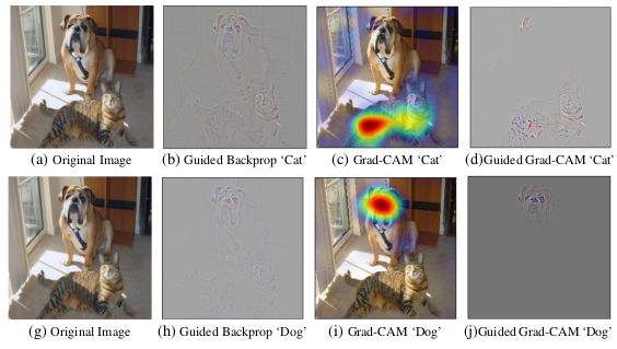
Figure 2: Different outputs of the explained algorithms for the same image but 2 different classes $y^c$.Notice how Guided Grad-CAM removes cat features over the dog face by combining the Guided Backprop result with the Grad-CAM result.
Results
Localization
In an image classification context, from the Grad-CAM maps the authors built the bounding box of the object being detected. They then measure the classification and localization score on ILSVRC-15 dataset for different architectures (VGG-16, AlexNet, GoogleNet). Results show that Grad-CAM (when compared to CAM) achieves lower location errors without compromizing on performance as CAM does by needing network modifications and re-training.
Segmentation
They replace the CAM component in the object segmentation task presented in this work by Grad-CAM, obtaining an increase of 5 percentage points in IoU score in Pascal VOC 2012.
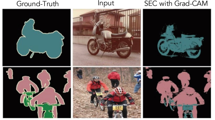
Figure 2: Segmentation result example
Discrimination
This experiment consisted in showing humans Guided BackProp and Guided Grad-CAM results for different images and labels from Pascal VOC 2007. The human’s task was to identify what label the model was guessing from the highlighted pixels. Results show that humans correctly identify 61.23% of Guided Grad-CAM labels and only 44.44% of Guided BackProp ones.
Trust
This experiment consisted in showing to humans model guesses and both Guided BackProp and Guided Grad-CAM outputs. These outputs show what regions in the image is the model basing its guesses. Again, human found Guided Grad-CAM regions of interest to be more trustworthy than Guided backprop.
Analyzing failure cases
This experiment consists on taking wrong network guesses and running the Grad-CAM algorithm to see what made the network thing of the wrong label. Results show that seemingly unreasonable predictions have reasonable explanations.
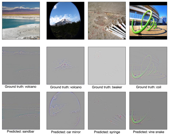
Figure 3: Failure examples and their explanation.
Adversarial noise
In this experiment the authors feed adversarial examples to some trained classification ANN. Later, they use Grad-CAM to highlight the areas of the correct labels. Results show that, even the guess is flawed due to the adversarial attack, the model is still able to recognize the correct entities in the image.
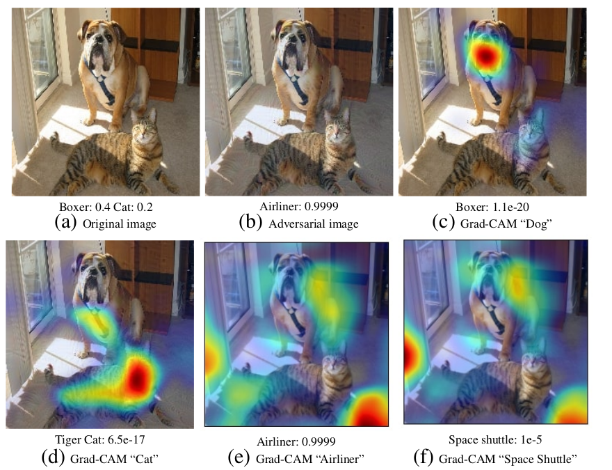
Figure 4: Adversarial attack Grad-CAM analysis.
Bias identification
Grad-CAM can also be used for bias identification in datasets. In this experiment the authors collected a set of images of 2 categories: doctor and nurse from “some popular image search engine”. They trained a CNN-based models to label those images and got a test accuracy of 82%.
Subsequently, they used Grad-CAM to analyse what the model was looking at. They noticed that the model had learned to look at the persons face (and hairstyle) to distinguish nurses from doctors, implicitly learning a gender stereotype. By analyzing the dataset the model was trained on, they discovered that 78% of images of doctors were men, while 93% of the images of nurse were women: The model had simply learn to take apart men from women.
By creating a new dataset (this time gender-unbiased) and re-training the model they achieved a better test accuracy (90%). This experiment can give an idea on how ANNs can inadvertedly become biased. This has big ethical outcomes as more decisions are being made based on this type of model guesses.
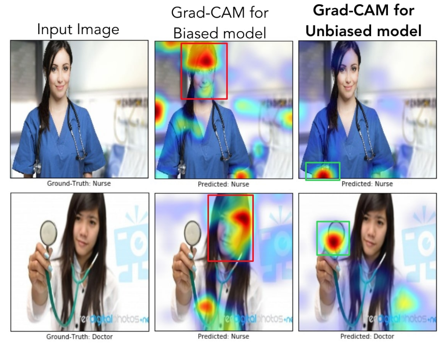
Figure 5: Dataset bias case example. Notice how the biased model is looking at the face of the person to guess its job, while the unbiased one is looking at the tools it has.
Image captioning and VQA
The authors show the adaptability of their approach to tasks different from classification. Again, Guided Grad-CAM outperforms Guided BackProp in all of them.
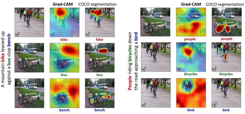
Figure 6: Captioning visualized with Grad-CAM.
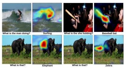
Figure 7: Visual Question Answering (VQA) visualized with Grad-CAM.
Contribution
-
Developed a more general visual explanation tool for CNN-based models
-
Show the usefulness of the approach on a wide variety of tasks.
Weaknesses
-
Still limited to networks which start with a CNN.
-
Future lines of work should bring explainability to other areas such as RL, NLP or video.