Understanding Black-box Predictions via Influence Functions
Idea
ANNs parameters are given uniquely from the data. But how do we know which data-points from our dataset are relevant?
Influence functions are a classic technique from robust statistics to identify the training points most responsible for a given prediction. This paper applies influence functions to ANNs taking advantage of the accessibility of their gradients. Its main claim is that “we can better understand model behavior by looking how it was derived from its training data”.
Notation:
- \(z_i = (x_i, y_i) \in \mathcal{D}\) is a data-point of the dataset.
- \(L(z, \theta)\) the model loss of that data-point for parameters \(\theta \in \mathbb{R}^p\).
- \(\hat \theta := \arg \min_\theta \frac{1}{n} \sum_i^n L(z_i, \theta)\) are the optimal parameters when training with the entire dataset (we assume all points have the same weight in the mean).
Initial assumptions: The loss function is twice-differentiable and convex in \(\theta\).
Upweighting a training point
The influence of upweighting \(z\) on the parameters \((I_{up, params}(z))\) tells us how are the training parameters going to change if the weight of given point \(z\) is increased by \(\epsilon\). I.e \(I_{up, params}(z) := \frac{\partial \hat \theta_{\epsilon, z}}{\partial \epsilon} \vert_{\epsilon=0}\). Where \(\hat \theta_{\epsilon, z} := \arg \min_{\theta} \frac{1}{n} \sum_i L(z_i, \theta) + \epsilon L(z, \theta)\)
Applying influence functions (and some Taylor-expansion approximations) we get:
\begin{equation} I_{up, params}(z) = - H_{\hat \theta}^{-1} \cdot \nabla_\theta L(z, \hat \theta) \end{equation}
Where \(H_{\hat \theta} \in \mathbb{R}^{p \times p}\) is the Hessian of the loss function w.r.t \(\theta\). It can be inverted since its positive definite (PD), thanks to the convexity assumption. \(\nabla_\theta L(z, \hat \theta) \in \mathbb{R}^{p \times 1}\) is the gradient of the loss function w.r.t \(\theta\) evaluated at \(z\) with parameters \(\hat \theta\).
If we take \(\epsilon = - \frac{1}{n}\) we can see the effect on the parameters of removing a point \(z\) from the dataset: \(\hat \theta_{-z} \simeq \hat \theta - \frac{1}{n} I_{up, params}(z)\).
\(I_{up, loss} (z, z_{test}) = \frac{\partial L(z_{test}, \hat \theta_{\epsilon, z})}{\partial \epsilon} \vert_{\epsilon=0}\) then encodes “how important” a data-point \(z\) is to a test-point \(z_{test}\). Developing we get:
\begin{equation} I_{up, loss} (z, z_{test}) = - \nabla_\theta L(z_{test}, \hat \theta)^T \cdot H_{\hat \theta}^{-1} \cdot \nabla_\theta L(z, \hat \theta) \end{equation}
Perturbing a training point
Using a similar reasoning, we can evaluate the influence a perturbation of some data-point \(z\) can have on the loss of some test-point \(z_{test}\):
\begin{equation} I_{pert, loss} (z, z_{test}) = - \nabla_\theta L(z_{test}, \hat \theta)^T \cdot H_{\hat \theta}^{-1} \cdot \nabla_x \nabla_\theta L(z, \hat \theta) \end{equation}
If we perform a \(\delta\) perturbation to \(z\), \(I_{pert, loss} (z, z_{test}) \cdot \delta\) tells us the effect it has on the loss of \(z_{test}\).
We can construct training-set attacks by choosing a small perturbation which augments test data loss._
\(I_{pert, loss} (z, z_{test})\) can also help us identify the key features of data-point \(z\) responsible for the prediction of \(z_{test}\).
Assumptions and approximations
There are 2 main drawbacks of directly using these expressions:
- Computing and inverting the Hessian is too expensive: \(O(n p^2 + p^3)\).
- We usually will want to compute \(I_{up, loss} (z_i, z_{test}) \forall z_i \in \mathcal{D}_{train}\).
These problems can be addressed using implicit Hessian-vector products (HVPs). Instead of explicitly computing \(H_{\hat \theta}^{-1}\) we can approximate \(s_{test} \simeq \nabla_\theta L(z_{test}, \hat \theta)^T \cdot H_{\hat \theta}^{-1}\) and then: \(I_{up, loss} (z, z_{test}) \simeq s_{test} \cdot \nabla_x \nabla_\theta L(z, \hat \theta)\). The authors consider two methods for approximating \(s_{test}\): conjugate gradients (CG) (exact but slower) and stochastic estimation (approx. but faster).
Results
-
Influence functions vs leave-one-out: Authors compare the proposed theoretical value of: \(- \frac{1}{n} I_{up, loss} (z, z_{test})\) vs actually training the system without that training-point: \(L(z_{test}, \hat \theta_{-z}) - L(z_{test}, \hat \theta)\). Both results math closely.
-
Non-convexity and non-convergence: Usually ANN training is done with SGD with early stopping or non-convex objectives. Let \(\tilde{\theta}\) be the found params. It can be that \(\tilde{\theta} \not ={\hat \theta}\), then \(H_{\tilde{\theta}}\) could have negative eigenvalues. Nevertheless, results show that the influence functions still give meaningful values.
-
Non-differentiable losses: Results show that smooth approximations of non-differentiable losses can still correctly guess the influence functions.
Contribution
The proposed method has many use-cases:
-
Understanding model behavior by telling which training points are responsible for certain behaviors.
-
Adversarial training examples: Models which place a lot of influence on small number of data-points are more vulnerable to training-input perturbations. Previously, adversarial attacks have been done in test inputs, the authors show that using influence functions they can also be done through test-inputs. In a dog vs fish classification task, they were able to flip the guess of 77% of labels by creating datasets with just 2 altered images.
-
Debugging domain mismatch: Influence functions help identifying when training distribution is different from testing distribution by detecting the test-points most responsible for errors.
-
Fixing mislabeled examples: The author set up this experiment: In a classification task, randomly flip 10% of labels and train a model. Then they try to find the flipped labels by the following methods: Finding the highest influence training-points with influence functions, finding the highest-loss and random. Results show that using influence function is the fastest way to both detect mislabelled data and improve test accuracy of themodel:
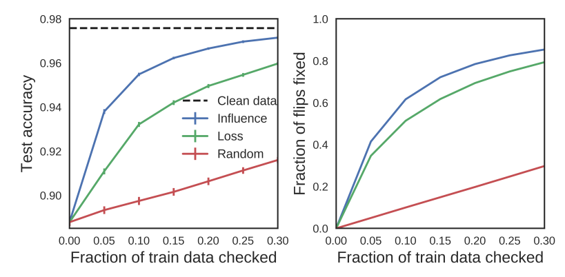
Figure 1: Proportion of train data which needs to be checked in a 10% mislabelled set depending on the chosen approach.
Weaknesses
-
Future line of work could tackle how sub-sets of training points affect the model. Not just how individual data-points locally affect the model performance.
-
I guess they fix the random seed but they don’t talk about the effect of different weight initialization and don’t seem to check how robust the results are to it.