A Simple Baseline for Bayesian Uncertainty in Deep Learning
This paper proposes the SWA-Gaussian algorithm for uncertainty representation and calibration in Deep Learning. Standard Neural Networks do not provide any information about the confidence of their predictions. The SWAG algorithm proposed in this paper achieves efficient Bayesian inference that performs better than other methods in both accuracy and calibration.
The SWA algorithm
In the SWA paper, Izmailov et al., 2019 the authors proposed the SWA -Stochastic Weight Averaging- procedure for training Deep Neural Networks, that leads to better generalization than standard training methods. In SWA, training is performed with the common Stochastic Gradient Descent technique, but in the final phase, an high or cyclical learning rate is used. After each epoch or cycle, the resulting model is kept, and the final model is given by the average of a window of the last models.
As conjectured by Chaudhari et al., 2017 and Keskar et al., 2017, local minima that are located in wide valleys of the loss function are better for generalization. However, SGD solutions often lie on the boundaries of these regions. This can be clearly seen in Figure 1: the SGD trajectory explores points on the boundaries of the optimal with respect to the test error. It becomes then desirable to average these points.
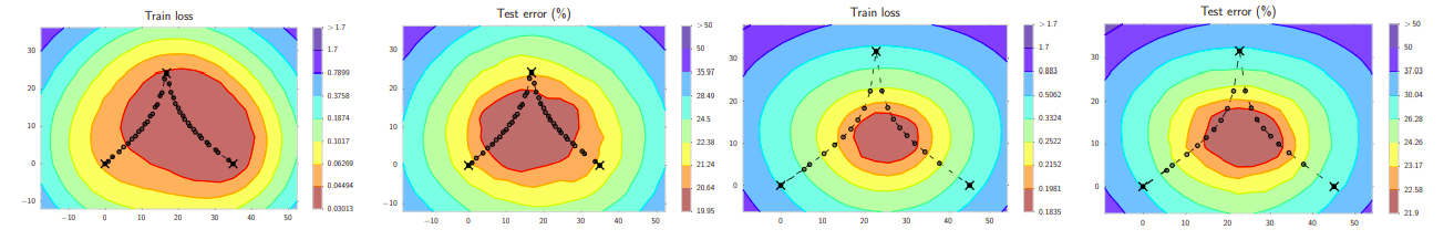
The L2-regularized cross-entropy train loss and test error surfaces of a Preactivation ResNet-164 on CIFAR100 in the plane containing the first, middle and last points (indicated by black crosses) in the trajectories with (left two) cyclical and (right two) constant learning rate schedules. Picture from the SWA paper.
Bayesian methods
Differently from the maximum likelihood methods, in the model parameters \(\theta\) are obtained as a point estimate of the ML solution for the dataset \(\mathcal{D}\)
\[\theta^{\star} = \arg\max_{\theta} \Big( \ln P(\mathcal{D} \vert \theta) + \ln p(\theta) \Big)\]in Bayesian methods we are interested in obtaining a distribution \(p(\theta \vert \mathcal{D})\) over these parameters. This allows us to perform Bayesian Model Averaging, i.e. do predictions by marginalizing the parameters
\begin{equation} \label{eq:bayes_avg} p(y_{\star} \vert x_{\star}, \mathcal{D}) = \int p(y_{\star} \vert x_{\star}, \theta) p(\theta \vert \mathcal{D}) d\theta \end{equation}
This paper proposes an extension to the SWA algorithm that also computes a covariance matrix over the model parameters.
The SWA-Gaussian algorithm
The work of Mandt et al., 2018 shows that Stochastic Gradient Descent simulates a Markov chain with a stationary distribution. The SWA algorithm computes the mean of this distribution. The SWA-Gaussian computes also the covariance matrix.
Diagonal covariance
To compute an approximation of the diagonal covariance of the SGD iterates the paper exploits the fact that \(Var(X) = E[X^2] - E[X]^2\). In our case, we have \begin{equation} \Sigma_{diag} = diag(\overline{\theta^2} - \theta_{SWA}^2) \end{equation}
where \(\overline{\theta^2}\) estimates the second uncentered moment of the distribution as \(\overline{\theta^2} = \frac{1}{T} \sum_{i=1}^T \theta_i^2\) and \(\theta_{SWA}\) is the SWA solution, i.e. the mean of the SGD stationary distribution \(\theta_{SWA} = \frac{1}{T} \sum_{i=1}^T \theta_i\)
Low rank plus diagonal covariance
A Diagonal covariance may be restrictive, therefore the paper provides a way of estimating the full covariance matrix. Being \(\{\theta_i\}_{i=1\: ... \:T}\) the models resulting from the SGD steps, the covariance matrix could be computed as \begin{equation} \Sigma = \frac{1}{T} \sum_{i=1}^T (\theta_i - \theta_{SWA})(\theta_i - \theta_{SWA})^T \end{equation}
During training, however, we do not have access to the value of \(\theta_{SWA}\), therefore the covariance matrix is approximated by \begin{equation} \Sigma \approx \frac{1}{T - 1} \sum_{i=1}^T (\theta_i - \overline{\theta}_i) (\theta_i - \overline{\theta}_i)^T = \frac{1}{T-1}DD^T \end{equation}
where \(\overline{\theta_i}\) is the running average of the first \(i\) samples, and \(D\) is the Deviation Matrix containing \((\theta_i - \overline{\theta_i})\) in the columns. A full-rank covariance matrix would scale quadratically with the model parameters, therefore the paper proposes to limit the rank of \(D\) by using only the last \(K\) models, obtaining \(\hat{D}\). The low-rank approximation is therefore given by \begin{equation} \Sigma_{low-rank} = \frac{1}{K - 1} \hat{D}\hat{D}^T \end{equation} and the resulting posterior distribuion of the parameters \(\theta\) is a Gaussian with mean \(\theta_{SWA}\) and covariance given by the sum \(1/2 (\Sigma_{diag} + \Sigma_{low-rank})\). Thus, the posterior is \begin{equation} \label{eq:posterior} p(\theta \vert \mathcal{D}) = \mathcal{N}\Big(\theta_{SWA}, \frac{1}{2}(\Sigma_{diag} + \Sigma_{low-rank})\Big) \end{equation}
Bayesian Model Averaging
Predictions are performed by marginalising over the parameters \(\theta\) as in Eq. \ref{eq:bayes_avg}. In practice, the marginalization is performed by Monte Carlo sampling \begin{equation} p(y_{\star} \vert x_{\star}, \mathcal{D}) \approx \frac{1}{T} \sum_{t=1}^T p(y_{\star} \vert x_{\star}, \theta_t), \end{equation} where \(\theta_t\) are sampled from \(p(\theta \vert \mathcal{D})\) of Eq. \ref{eq:posterior}. To efficiently sample from \(p(\theta \vert \mathcal{D})\) we can exploit the identity \begin{equation} \tilde{\theta} = \theta_{SWA} + \frac{1}{\sqrt{2}} \Sigma_{diag}^{\frac{1}{2}} z_1 + \frac{1}{\sqrt{2(K - 1)}} \hat{D} z_2 \end{equation} where \(z_1 \sim \mathcal{N}(0, I_d)\) with \(d\) being the number of parameters in the network, and \(z_2 \sim \mathcal{N}(0, I_K)\).
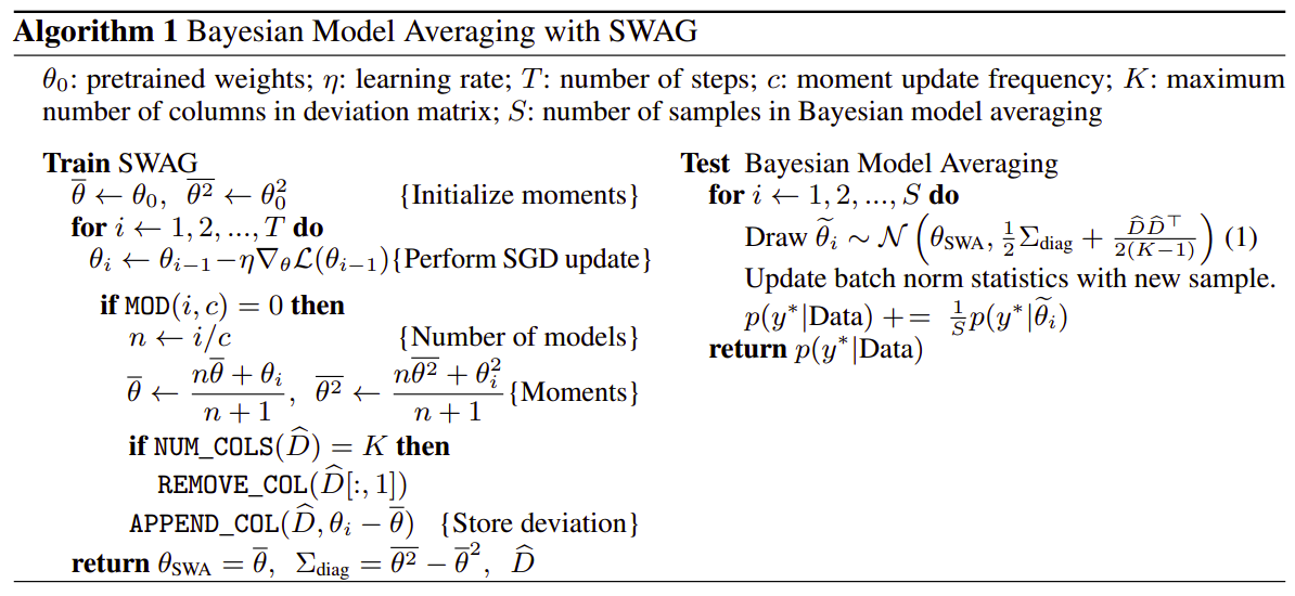
The SWAG algorithm training and testing
Results
The paper evaluates SWAG by comparing it with several state-of-the-art baselines, such as MC dropout, Temperature Scaling, SGLD, Laplace approximations, Deep Ensembles, and ensembles of SGD iterates that were used to construct the SWAG approximation.
-
Classification: SWAG performs better than all other methods tested in computer vision classification tasks in terms of accuracy on CIFAR and ImageNet datasets.
-
Calibration: SWAG and SWAG-Diagonal perform comparably or better than all the other methods testes in calibration tasks. Calibration is measured as the difference between the confidence of the network and its the actual accuracy.
-
Out-of-domain image detection: SWAG and SWAG-Diagonal are better than the other methods in recognising data that does not belong to the known classes in image classification tasks.
Contributions
-
The paper proposes the SWAG algorithm, that turns the successful SWA algorithm into an efficient and tractable Bayesian inference method. The computation of covariance and mean are performed once per epoch and their cost scale linearly with the model parameters.
-
The paper provides extensive theoretical and empirical analysis of the technique, with the most important observation being that the posterior over weights is close to gaussian in the subspace spanned by the SGD trajectory.
-
The paper shows that Bayesian Model Averaging on the SWAG posterior performs often better than SWA and SGD.
-
The proposed SWAG algorithm can be useful in situations where, along with the prediction, one needs to know its confidence.
Weaknesses
- Although the training is comparably faster with SGD, the prediction step requires to sample several models and perform predicitons with each one. This may be negligible or not depending on the application.