Out-of-Distribution Detection Using an Ensemble of Self Supervised Leave-out Classifiers
Out-of-Distribution (OOD) Detection consists of being able to identify data that lies outside the domain a Deep Learning system had been trained with. This can include recognizing when an image does not belong to any of the known classes, detecting a sensor failure or a cyber attack. In this paper, the authors propose an OOD detection algorithm that exploits an ensemble of self-supervised classifiers trained by using a partition of the data as OOD data. The proposed algorithm outperforms the state-of-the-art ODIN.
Idea
Softmax outputs of classifiers are often seen as output probabilities for each class. However, Chang Guo et al., 2017 show that this is not often the case, in particular when predicting inputs outside the range of training data. We cannot therefore rely on softmax to estimate prediction uncertainty or out-of-distribution detection. This paper proposes a technique to make the softmax predict with high entropy for out-of-distribution data and with low entropy for in-distribution data. This is achieved by training an ensemble of classifiers, each one using a partition of the classes as out-of-distribution data, with an entropy based loss function.
Entropy based margin loss
This paper proposes a modified loss function for the classifiers training. Given a dataset of in-disttribution samples \((x_i \in X_{in}, y_i \in Y_{in})\) and out-of-distribution samples \(x_o \in X_{ood}\), this loss term aims to maintain a margin of at least \(m\) between the average entropy of predictions for in and out distribution. Being \(F: x \rightarrow p\) the Neural Network function that maps an input \(x\) to a distribution over classes, the loss is given by
\begin{equation} \mathcal{L} = -\frac{1}{\vert X_{in} \vert} \sum_{x_i \in X_{in}} \ln(F_{y_i}(x_i)) \underbrace{+\beta \max \Bigg( m + \frac{\sum_{x_i \in X_{in}}H(F(x_i))}{\vert X_{in}\vert} -\frac{\sum_{x_o \in X_{ood}}H(F(x_o))}{\vert X_{ood}\vert}, 0 \Bigg)}_{entropy-margin} \end{equation}
This loss function is made of two terms: the corss-entropy loss and the novel entropy-margin loss. The first makes the classifiers correclty classify data points, while the second encourages it to predict softmax scores with high entropy for out-of-distribution inputs, and low entropy for in-distribution inputs.
\(F_{y_i}(x_i)\) represents the predicted probability of class \(y_i\) for input \(x_i\), while \(F(x)\) represents the whole output distribution for input \(x\), and thus \(H(F(x_i))\) is the entropy of the softmax scores.*
High entropy softmax scores means that the predicted softmax values are approximately equal for all classes, while low entropy scores means that the highest softmax value will be much higher than the others.*
Bounding the second loss term by a marging \(m\) is helpful in reducing overfitting. Without it the classifiers could easily overfit in assigning high entropy to the out-of-distribution training data partition at the cost of not generalizing to other unseen data. Keep in mind that this out-of-distribution data is not really out of distribution as it is part of the dataset.*
Training the ensemble
The training data \(X\) is divided into \(K\) mutually-exclusive partitions \(\{X_i\}_{i=1}^K\), i.e. no classes are contained by more than one partition. For each partition \(X_i\), a classifier \(F_i\) is learned by using \(X_i\) as out-of-distribution data and the rest of data partitions as in-distribution data. The process is described in Algorithm 1.
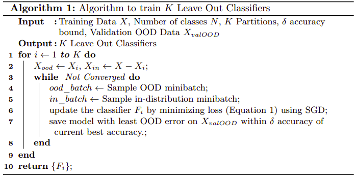
Learning K classifiers using a different partition as out-of-distribution data each
Classification
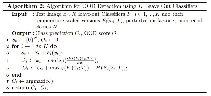
In classification, the input \(x\) is fed to all the \(K\) classifiers, and the output softmax vectors -that have size \(K-1\) since one class was left out as out-of-distribution data- are resized to length \(K\). A zero is set at the left out class position. The softmax vectors are then averaged and the resulting \(\arg\max\) is used for classification, as shown in Algorithm 2.
Out of Distribution Detection
When computing the OOD Detection scores, temperature scaling and input preprocessing are applied.
Temperature scaling is used when computing the softmax over the output logits. In temperature scaling, the logits of the classifier output are divided by a constant temperature parameter \(T\) before being fed to the softmax. It has been empirically shown by Liang et al., 2020 that temperature scaling pushes softmax outputs apart for in and out of distribution data.
Input preprocessing consists in adding a small perturbation against the entropy loss, according to Eq. \ref{eq:preproc}. \begin{equation} \label{eq:preproc} \tilde{x} = x - \epsilon \ \text{sign} \Big(\frac{\partial \mathcal{L}(F_{i}(x, T))}{\partial x} \Big) \end{equation} This perturbation decreases the entropy of the in-distribution samples more than that of the out-of-distribution samples. This is inspired from Goodfellow et al., where small perturbations of the input are applied to decrease the softmax activation of the correct class and force the classifier to a wrong prediction.
There are some weaknesses in the temperature scaling and input preprocessing approach that I discuss in the Weaknesses section.
Finally, OOD Detection scores are computed by feeding the input to all \(K\) classifiers (using temperature scaling and input preprocessing). For each of the resulting softmax vector, the maximum value and negative entropy are computed and the OOD Detection score is given by the sum of the max values and negative entropies, as shown in Algorithm 2. These values are important since in-distribution and out-of-distribution samples will behave differently:
-
In-distribution samples: Every in-distribution sample \(x_i\) with (unknown) class \(y_i\) acts as out-of-distribution for exactly one classifier. Therefore, we expect \(K - 1\) classifiers to output an high maximum softmax value with high negative entropy (the model will be more confident in the prediction). For the same reason, we expect the classifier for which \(y_i\) was left out to output low maximum value and low negative entropy.
-
Out-of-distribution samples: We expect an out-of-distribution sample to produce low maximum value and low negative entropy for all the \(K\) classifiers.
It is not clear from the paper how these OOD Detection scores are effectively used.*
Results
The algorithm is trained using the CIFAR-10 and CIFAR-100 image datasets. Then the test is performed on different datasets such as TinyImageNet, LSUN, iSUN, and synthetic noises.
-
The proposed algorithm performs better than the previous state-of-the-art, ODIN in terms of false positive rate, detection error (see the ODIN paper for definition), and many other metrics.
-
The ODIN algorithm remains superior in OOD Detection for synthetic datasets, where the proposed algorithm performs poorly.
-
Ablation study show that in CIFAR-100, using 5 classifiers gives the best result, and 3 can also be a good trade off between performances and computational cost. They also show that temperature scaling and input preprocessing are effective.
Contributions
-
The paper proposes a new state-of-the art approach to Out-Of-Distribution Detection.
-
The proposed loss opens an interesting and promising area of work, based on the entropy of the predictions. Research could be done to find the best ways of producing predictions with different entropies for in and out of distribution data.
-
The ensemble of leave-out classifiers stands as a promising approach for this type of tasks. It has the benefit of using the whole dataset, but at the same time using part of it as out-of distribution data.
-
This paper leaves other research questions open: can the proposed ensemble be distillated Manilin et al., 2019? What is the relation between this approach and uncertainty estimation techniques in Neural Networks Blundell et al., 2015, Lakshminarayanan et al., 2017?
-
The algorithm has been tested on a wide range of network architectures and with a large and diverse set of out-of-distribution datasets.
Weaknesses
Some practical weaknesses of this paper:
-
The ensemble has high memory requirement and an high computational cost. All the \(K\) models need to be kept in memory, which for big networks may not be ideal. Moreover, the training time of one classifier is multiplied by \(K\), and the same applies for classification. The OOD Detection requires additional \(K\) inferences to be performed. This may not be ideal in real-time OOD Detection, which includes many useful applications such as detecting sensor failures or cyber attacks.
-
The paper is quite unclear on how the OOD Detection scores should be used in detecting out-of-distribution data. It describes how those scores are computed, but not how the treshold between in and out distribution is decided.
And some more theoretical ones:
-
The paper, among other things, relies on temperature scaling, which was successfully employed also by the ODIN paper. However, this technique does not rely on solid theoretical grouds. First, the ODIN paper approximates a first order Taylor expansion of the temperature-softmax. Then, they extrapolate two terms, \(U_1\) and \(U_2\) from this approximation, i.e. \(S(x, T) \propto \frac{U_1 - U_2/2T}{T}\). \(U_1\) “measures the extent to which the largest unnormalized output of the neural network deviates from the remaining outputs”. \(U_2\) instead “e U2 measures the extent to which the remaining smaller outputs deviate from each other”. Then, they show that the effect of T is of increasing the relative weight of \(U_1\) with respect to \(U_2\). The authors then perform empirical observations about the distribution of \(U_1\) and \(U_2\) on their in-distribution dataset (CIFAR-100) and their out-of-distribution datasets (CIFAR-10&100, iSUN, ImageNet, LSUN), and observe that \(U_1\) is higher for in-distribution data. The whole technique therefore relies on the empirical evidence for the datasets in consideration, but there is no guarantee that the same conditions will apply to other datasets or type of data. The paper I analyze in this article also employes the trick successfully, but since it uses the same datasets, we cannot draw any different conclusion.
-
The paper employes also the input preprocessing technique. The ODIN paper used it to noise the input in the direction of the cross-entropy loss gradient, thus tricking the network into assigning higher value to the predicted class. This, again, does not rely on solid grouds, as it is based on the same empirical study of above and thus closely related to the datasets in consideration. However, this paper uses a different version of the technique, that noises the image in the direction of the entropy loss gradient. The authors state “Perturbing using the entropy loss decreases the entropy of the ID samples much more than the OOD samples”, but it is not clear on what evidence does this rely.
-
The algorithm has an important downside: it performs poorly on synthetic noise datasets (uniform and gaussian) with, depending on the architecture, false positive rate up to 99.9%. This is clearly an important shortcoming, as it suggests that the algorithm is able to detect out-of-distribution samples that are still in some way similar to the in-distribution data (e.g. images coming from other datasets) but not samples that are very different from the in-distribution. I hypothesize that this is due to using similar data as out-of-distribution in the loss function. Maybe an adversarial training, where an adversarial network learns to generate OOD samples that the classifiers cannot detect and use those in the entropy-margin loss could overcome the problem?