Generalized Cross Entropy Loss for Training Deep Neural Networks with Noisy Labels
A central issue in standard Deep Neural Network training for classification tasks is the need of large datasets of labeled samples. While collecting data is often cheap and fast, the labeling process is much more expensive and difficult. In many cases, however, we can obtain such a dataset at smaller cost, but with noisy labels, i.e. labels that have a certain probability of being wrong.
Noisy labels can degrade Deep Neural Networks performance. Therefore, in the last year many researchers focused on finding ways of training DNNs in presence of noisy labels. One field of this research is finding loss functions that are robust to such noise. This paper proposes a family of noise-robust loss functions whose behavior spans between the Mean Absolute Error (MAE) loss and the Categorical Cross Entropy (CCE) loss.
Background
Let \(X\) be the feature space and \(Y = \{1, ..., c\}\) the label space. For a given sample \(x_i\), the correspondent label \(y_i\) is represented in the common one-hot encoding. A clean dataset \(\mathcal{D} = \{(x_i, y_i)\}_{i=1}^n\) is a dataset with correct labels \(y_i\). Let \(f(\theta, x)\) be the Neural Network function parametrized by \(\theta\) that maps \(x\) to the predicted label \(y\). In this article we always assume that the last layer of \(f\) is a softmax layer, therefore \(f(\theta, x) \in [0, 1]^{c}\) always.
Notation
In this article \(f(x)\) is always intended to be parametrized by \(\theta\), i.e. \(f_{\theta}(x) = f(x)\). \(f_j(x)\) represents the \(j\)-th output of the softmax classifier \(f\). \(f_{y_i}(x_i)\) represents the output for the true label specified by \(y_i\), which is a \(c\)-dimensional one-hot encoding vector. The loss function \(\mathcal{L}(f(x), j)\) is intended to be the loss for sample \(x\) when the ture label is class \(j\). Occasionally it may be written as \(\mathcal{L}(f(x_i), y_i)\). In this case the loss is intended as the loss of sample \(x\) when the true label is the one specified by \(y_i\).
Empirical Risk
The empirical risk \(R_{\mathcal{L}}(f)\) of the classifier \(f\) for a loss function \(\mathcal{L}\) is defined as the expected value of \(\mathcal{L}\) over the empirical distribution \(p_{D}(x_i, y_i)\): \begin{equation} R_{\mathcal{L}}(f) = E_{p_{D}(x, y)}\left[\mathcal{L}(f(x), y)\right] \end{equation} The goal of a learning algorithm is, generally, to minimize the risk over the real data distribution by minimizing the empirical risk.
More about the Risk Minimization Framework in Goodfellow et al., Deep Learning, Section 8.1.1 and Vapnik, Principles of Risk Minimization for Learning Theory
Noisy Dataset
A noisy dataset \(\mathcal{D}_{\eta} = \{(x_i, \tilde{y}_i)\}_{i=1}^n\) is a dataset with noisy labels \(\tilde{y}_i\), which the paper assumes to be independent of inputs given the true label, i.e.
\[p(\tilde{y}_i = k \vert y_i = j, x_i) = p(\tilde{y}_i = k \vert y_i = j) = \eta_{jk}\]which is class dependent. The risk of classifier \(f\) with respect to this dataset is \(R^{\eta}_{\mathcal{L}}(f) = E_{p_{\mathcal{D}_{\eta}}(x, \tilde{y})}\left[\mathcal{L}(f(x), \tilde{y})\right]\).
The noise is uniform when the probability of a correct label is equal to \(1 - \eta\) and the probability of a wrong label is uniformly distributed among the remaining classes, i.e.
\[p(\tilde{y} = k \vert y = j) \begin{cases} 1 - \eta & \text{if } k = j\\ \frac{\eta}{c - 1}, & \text{if }k \ne j \end{cases}\]Noise Tolerant Loss Functions
Let \(f^*\) be the global minimizer of \(R_{\mathcal{L}}(f)\), the empirical risk on the clean dataset. A loss function is said to be noise tolerant if \(f^*\) is also a global minimizer of \(R_{\mathcal{L}}^{\eta}\), the empirical risk on the noisy dataset.
As proved in Gosh et al., 2015, Making Risk Minimization Tolerant to Label Noise, if the loss function \(\mathcal{L}\) is symmetric and \(\eta < \frac{c-1}{c}\) then, under uniform noise, \(\mathcal{L}\) is noise tolerant. Additionally, if \(R_{\mathcal{L}}(f^*) = 0\), then \(\mathcal{L}\) is noise tolerant under class dependent noise.
A loss function is symmetric if exists a value \(C\) such that \begin{equation} \sum_{j=1}^c \mathcal{L}(f(x), j) = C \end{equation} for every \(f\) and \(x\). An example of symmetrical loss function is the Mean Absolute Error (MAE):
The final result is obtained by the fact that the last layer of f is a softmax, and thus \(f\ge0\) and \(\sum_{k=1}^c f_k(x) = 1\). \(e_j \in \{0, 1\}^c\) is the canonical basis vector with 1 in the \(j\)-th element and 0 everywhere else.
However, despite having the nice property of being noise tolerant, MAE loss performs poorly. On the other hand, Categorical Cross Entropy,
is not simmetrical neither bounded, and therefore sensitive to noisy labels, but is known to perform well in clean datasets. The paper compares CCE and MAE losses in the (clean) CIFAR datasets, and the CCE loss is shown to lead to better performances.
\(y_{ij} \in \{1, ..., c\}\) is 1 if the true label of sample \(i\) is \(j\) and 0 otherwise.
Idea
The first idea of the paper is to combine the noise tolerancy of MAE loss with the effectiveness of CCE loss.
Generalized Cross Entropy Loss
The paper proposes to use the Box-Cox transformation as a loss function: \begin{equation} \mathcal{L}_{q}(f(x), j) = \frac{1 - f_j(x)^q}{q} \end{equation} where \(q \in [0, 1]\) is a tuning parameter. By computing the limits we observe that for \(q=0\) the \(\mathcal{L}_q\) loss becomes the CCE loss, while for \(q=1\) it becomes the MAE loss up to a multiplicative constant. Therefore, this loss provides a trade-off between noise tolerancy -\(q\) close to 1- and performances -\(q\) close to 0-, and can be seen as a generalization of both. The gradient is:
\[\nabla_{\theta}\mathcal{L}_q (f(x), j) = -f_j(x)^{q-1}\nabla_{\theta}f_j(x)\]that can be seen as a weighted gradient with weight given by the factor \(-f_j(x)^{q-1}\) tuned by \(q\). The closer \(q\) is to 0, the more weight is given to samples for which \(f\) predicts a low softmax value for the correct class \(j\). At \(q=0\) the gradient is the same of CCE loss. For values of \(q\) closer to 1, the gradient is the same of MAE loss and the same weight is given to every sample gradient.
Truncated Loss
The paper proves that a truncated version of the loss above is more tolerant to noise. For a threshold parameter \(k \in [0, 1]\), the truncated loss \(\mathcal{L}_{trunc}\) is given by:
\[\mathcal{L}_{trunc}(f(x), j) = \begin{cases} \mathcal{L}_q(k) & \text{if } f_j(x) < k \\ \mathcal{L}_q(f(x), j) & \text{if } f_j(x) \ge k \\ \end{cases}\]where \(\mathcal{L}_q(k) = \frac{1 - k^q}{q}\). The parameter \(k\) acts as a threshold. If the softmax output for the correct class is smaller thank \(k\), the loss is constant with respect to \(\theta\). Therefore, the gradient will be zero, and the sample will effectively not count. Ideally, the higher the noise in the dataset, the closer \(k\) should be.
It is however not a good idea to directly use this loss for training when values of \(k\) are high, e.g. \(k = 0.5\). In fact, very few samples will have high softmax outputs in the beginning of the training. The classifier would be therefore trained only on a small subset of samples. To circumvent the issue, the paper shows that optimizing the truncated loss is the same as solving the following:
The weights \(w \in \{0, 1\}^n\) determine which samples are used. \(w\) and \(\theta\) are alternately optimized using the alternative convex search (ACS) algorithm. The update of \(w\), called pruning, is performed by computing \(f_{y_i}(x_i)\) for each training sample, and keeping (\(w_i\) = 1) only those with \(f_{y_i}(x_i) \ge k\) and \(\mathcal{L}_q(f(x_i), y_i) \le \mathcal{L}_q (k)\).
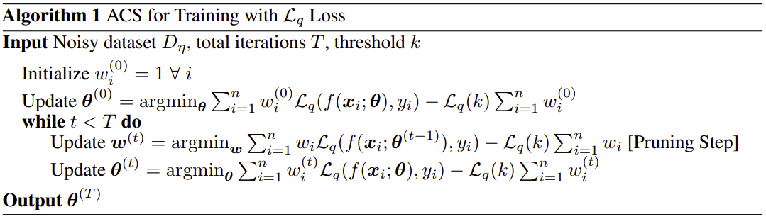
Figure 1: The ACS algorithm to train the weighted loss. Figure from the paper.
Does this really improve on the truncated loss? See the Weaknesses section for my thoughts.
Results
A ResNet is trained for different values of \(q\) and noise \(\eta\) on the CIFAR-10 dataset. Only the training and validation datasets are corrupted with noise, while the test set is left with the true labels.
-
When trained without noise (\(\eta=0\)), higher values of \(q\) show worse performance on the test set, and the best are for\(q=0\), i.e. the standard CCE loss.
-
By increasing the noise \(\eta\) to 0.2 and 0.6 the test accuracies decrease for low values of \(q\), while the best results are obtained for values \(q = 0.8\) and 1.0.
-
The validation plots suggest that low values of \(q\) make the network overfit to the noisy datasets, while this does not happen with higher values.
A comparison between \(\mathcal{L}_q\) loss and truncated loss, pure CCE and MAE losses, and other noisy-labels techniques is performed for uniform and class-dependent noise. \(q\) is kept fixed at 0.7. While \(\mathcal{L}_q\) loss and truncated loss are among the best in uniform noise datasets, they do not always provide the same performances in class dependent noise. In particular, Forward T (Patrini et al., 2017, Making Deep Neural Networks Robust to Label Noise: a Loss Correction Approach) perform consistently better in class-dependent noise datasets.
An open set noise is build by introducing some images from CIFAR-100 into CIFAR-10 and assigning them a random CIFAR-10 class. When tested in this dataset, the truncated loss provided the best accuracy among all the above methods.
Contribution
-
The paper proposes a generalized class of loss functions whose behavior spans between MAE and Categorical Cross Entropy, and can be tuned with a single parameter. The paper further develops on how to train with such a loss, providing an Alternate Convex Search algorithm that at each step trains the network on a subset of the training samples. This subset is computed by pruning the training set from all samples that are likely to be noisy.
-
The paper shows how the theory developed by Gosh et al. can be exploited to construct novel noise tolerant loss functions. It provides bounds of the expected risk for the proposed loss. In doing so, it explains the procedure, that can be used to develop other loss functions robust to noise. The theorems in the Appendix provide extensive theoretical results on properties of this family of loss functions.
-
The paper pushes the research in an area that, to the best of my knowledge, received little attention. While lot of work is being done in developing methods to perform classifiaction on noisy datasets, little attention has been given to building noise-tolerant loss functions.
Weaknesses
The major weaknesses are related to the ACS algorithm, and the experiments.
Weaknesses in weighted loss ACS
The weighted loss and the related ACS algorithm (both in Figure 1) is developed to overcome the issue of the truncated loss. The truncated discards, at each training step, every sample for which the softmax output of the true label is less than the threshold \(k\). I argue that the ACS algorithm of Figure 1 does the same. The paper in Section 3.3 says:
“At every step of iteration, pruning can be carried out easily by computing \(f(x_i)\) for all training samples. Only samples with \(f_{y_i}(x_i) \ge k\) and \(\mathcal{L}_q(f(x_i), y_i) \le \mathcal{L}_q(k)\) are kept for updating \(\theta\) during that iteration (and hence \(w_i = 1\)).”
I do not see any actual difference between this and the simple truncated loss alone. The truncated loss discards, at each training step, every sample for which \(f_{y_i}(x_i) \le k\). This algorithm does the same, as \(\mathcal{L}_q(f(x_i), y_i) < \mathcal{L}_q(k)\) implies \(f_{y_i}(x_i) > k\). Therefore both the truncated loss and the ACS algorithm discard the same set of samples. The difference is that while the truncated loss re-evaluates this condition every time, in the ACS algorithm this is done once, then \(\theta\) is optimized. This is then repeated for \(T\) iterations. It could be argued that samples that after a few optimization steps would be discarded by the truncated loss are kept more by the ACS algorithm. However, the contrary could also happen, i.e. samples that a few optimization steps would make usable could be discarded because of an initial zero weight. This could be even more true at the beginning of the training with high \(k\) threshold. Unfortunately, the paper does not provide any comparison between the simple \(\mathcal{L}_q\) loss, the truncated loss, and the ACS algorithm.
Suggestion for future research
Despite the weaknesses highlighted above, he ACS idea seems really interesting. Indeed, research should be done to compare it with the results that this paper provides for the \(\mathcal{L}_q\) loss. Moreover, it naturally leads to the idea of using continuous weights, and updating them with gradient techniques.
The ACS algorithm can also be viewed as a more general algorithm in which the two steps perform the operations of selection and optimization. The selection step selects the samples to use (by assigning weights, probabilities of sampling, or other methods). The rightmost term \(-\mathcal{L}_q(k) \sum_{i=1}^n w_i\) of the weighted loss can be seen more generally as a regularization term of the selection step, since it does not depend on \(\theta\). The optimization steps optimizes the network on the training set modified by the selection step.
Weaknesses in experiments
The paper compares ResNet training on CIFAR-10 for different values of \(q\) and noise \(\eta\) (Figure 2 in the paper). It would have been interesting to see the same comparison with the truncated loss and the weighted loss using ACS. In fact, this is the only experiment that explores different values of \(q\).
The following experiment -on CIFAR-10, CIFAR-100, Fashon MNIST- compare the \(\mathcal{L}_q\) and the truncated loss with CCE, MAE, and other noisy labels techniques. \(q\) is kept fixed to 0.7.It would have been interesting to see the comparison with also the ACS algorithm, especially to compare it with the truncated loss. It is also not clear the choice of \(q=0.7\), when the experiment described in the paragraph above suggested a value between 0.8 and 1.