So far we’ve seen:
- Standard RL: Learn an optimal policy (optimal action given a state) for a single task. I.e. fit network parameters for a given MDP:
-
Forward Transfer: Train on one task, transfer to a new one.
-
Multi-task learning: Train on multiple tasks, transfer to a new one.
The more varied the training, the more likely the transfer is to succeed.
These methods transfer knowledge either re-using a model of the environment (as we saw in model-based RL) or through a policy (requiring fine-tunning). What about transferring knowledge through learning methods though?
Introducing: Meta-Learning
Meta-learning refers to a learning to learn framework that leverages past knowledge to solve novel tasks more efficiently.
In generic supervised setting we have a single dataset \(\mathcal{D} = \left\{ \mathcal{D}^{tr}, \mathcal{D}^{test}\right\}\):
\begin{equation} \theta^\star = \arg \min_{\theta} \mathcal{L} (\theta, \mathcal{D}^{tr}) =: f_{\text{learn}} (\mathcal{D}^{tr}) \end{equation}
We can think of supervised training as a function $f_{\text{learn}} (\mathcal{D}^{tr})$ that, given a dataset, returns the parameters which minimize the functional form we assumed for our model on the train set.
In generic supervised meta-learning setting we have a set of datasets: \(\mathcal{D}_1, ..., \mathcal{D}_n\)
\begin{equation} \theta^\star = \arg \min_{\theta} \sum_i \mathcal{L} (\phi_i, \mathcal{D}^{test}_i) \end{equation}
Where
\begin{equation} \phi_i = f_{\theta} ( \mathcal{D}^{tr}_i ) \end{equation}
So a meta-learner attempts to find the lowest average test loss over all the different datasets (tasks) wrt post-adaptation parameters \(\phi_i\) obtained by running the learning adaptation procedure \(f_{\theta}\). So, in essence, we are learning \(f_\theta\), which is a way (a function) to learn model parameters for a given task.
A common way to implement it, is by using RNNs:
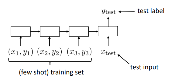
Implementation of meta-learning using a RNN approach.
If we try to express it as in the previous equations: the parameter vector produced by the adaptation process is the concatenation of the hidden state after seeing the dataset and the meta-learned weights. This means we can adapt to any new task by just computing the hidden state (RNN context) after running through that task training data.
\[\phi_i = \left[ h_i, \phi_p \right]\]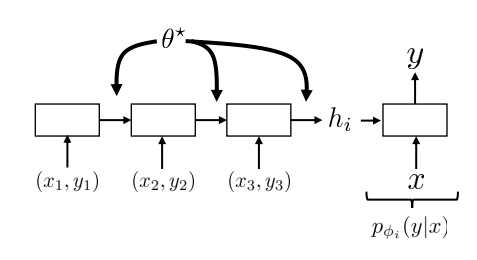
Main parameters of RNN as meta-learning technique.
Meta-Reinforcement Learning
Why is it a good idea? Using its past experience, a meta-learned learner can:
- Explore more intelligently
- Avoid trying useless actions
- Acquire the right features more quickly
Remember: In standard RL for an MDP: \(\mathcal{M} = \{ \mathcal{S}, \mathcal{A}, \mathcal{P}, r \}\) we learn the parameters of a model as:
\begin{equation} \theta^\star = \arg \max_\theta E_{\pi_\theta (\tau)} [ R( \tau ) ] =: f_{\text{RL}} (\mathcal{M}) \end{equation}
In Meta-RL, again we want to learn an adaptation procedure. If we have a set of MDPs: \(\mathcal{M} = \{ \mathcal{M}_1, ... \mathcal{M}_n \}\) that share some common structure (come from the same MDP prob distribution), we can learn some common parameters \(\theta\). This algorithm step is known as Meta-training or Outer loop:
\begin{equation} \theta^\star = \arg \max_\theta \sum_i E_{\pi_{\phi_i} (\tau)} [ R( \tau ) ] \end{equation}
From those, we can fit any individual related task with few samples. This means that for \(\mathcal{M}_i\), we will derive its optimal policy parameters \(\phi_i\) from the meta-learned ones. This algorithm step is known as Adaptation or Inner loop:
\begin{equation} \phi_i = f_\theta (\mathcal{M}_i) \end{equation}
This is different from contextual policies (multi-task RL) in the sense that the task context is not given, but inferred from experience of \(\mathcal{M}_i\)
The adaptation procedure has 2 main goals:
- Exploration: Collect most informative data
- Adaptation: Use that data to obtain the optimal policy.
The adaptation policy (defined by params \(\theta\)) does not need to be good at any task, only to be easily adaptable to all of them. We can think of \(\theta\) as a prior we’ll use to learn a posterior for each task.
In addition we are assuming all the train and test tasks are samples of some distribution of related MDPs: \(\mathcal{M}_i \sim p(\mathcal{M})\). In practice this is more of a technical assumption and its hard to proof until what degree it holds.
Meta-RL algorithms
The most basic algorithm idea we can try is:
While training:
- Sample task \(i\), collect data \(\mathcal{D}_i\)
- Adapt policy by computing: \(\phi_i = f(\theta, \mathcal{D}_i)\)
- Collect data \(\mathcal{D}_i^\prime\) using adapted policy \(\pi_{\phi_i}\)
- Update \(\theta\) according to \(\mathcal{L} (D_i^\prime, \phi_i)\)
Notice: Steps 1-3 belong to the adaptation step while step 4 belongs to the meta-training step.
Improvements:
- Run multiple rounds of the adaptation step
- Compute \(\theta\) update (step 4) across a batch of tasks.
From now on, we’ll mainly be discussing different choices for function \(f\) and loss \(\mathcal{L}\).
Recurrence algorithm
We want to collect new information while recalling what we’ve seen so far. Thus, it seems that encoding the policy as a RNN can be a good idea. Analogous as the RNN approach to supervised meta-learning, we can have the agent collect \((s, a, r)\) tuples as it interacts with the environment and use them to update its internal state:
.
As before, we have that \(\phi_i = \{ h_i, \theta \}\)
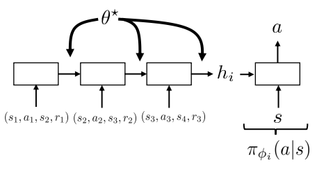
Crucially when training, we do not reset the internal state of the RNN between different episodes of the same MDP. Thus, the internal state is individual to each task but kept constant between different episodes of the same task. Optimizing the total reward of the entire meta-episode with an RNN policy automatically learns to explore.
Recurrent algorithm idea. In this case 2 meta-episodes are presented: One for MDP1 and one for MDP2.
Then the basic algorithm becomes:
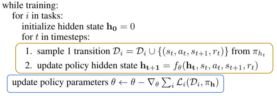
Recurrent algorithm pseudocode.
Pros/Cons:
- Conceptually simple.
- It is general and expressive: There exists and RNN that can compute any function.
- It is NOT consistent: There is no guarantee it will converge to the optimal policy.
- Vulnerable to meta-overfitting (can’t generalize to unseen tasks).
- Challenging to optimize in practice.
More on: Benchmarking Deep Reinforcement Learning for Continuous Control, Learning to reinforcement learn, A Simple Neural Attentive Meta-Learner and Efficient Off-Policy Meta-Reinforcement Learning via Probabilistic Context Variables.
Gradient-Based Meta-Learning
Gradient-Based Meta-Learning (aka Model-Agnostic Meta-Learning: MAML) main idea is to learn a parameter initialization from which fine-tunning for a new task works easily.
This is similar to when we pre-train a CNN with ImageNet to find good feature extractors and fine-tune with our given data.
Expressing it as in previous terms, we have that we are learning:
\begin{equation} \theta^\star = \arg \max_\theta \sum_i E_{\pi_{\phi_i} (\tau)} [ R( \tau ) ] \end{equation}
Where we define the adaptation parameters as a gradient step from the common parameters:
Remember that \(J_i (\theta) = E_{\pi_\theta} (\tau) [ R(\tau) ]\)
So, instead of learning the parameters that maximize the expected trajectory reward: \(\theta \leftarrow \theta + \alpha \nabla_\theta j(\theta)\) (as we would do in standard RL), we are learning the parameters which maximize the expected return of taking a gradient step for each task:
\begin{equation} \theta \leftarrow \theta + \beta \sum_i \nabla_\theta J_i \left[\theta + \alpha \nabla_\theta J_i (\theta)\right] \end{equation}
I.e: We want to find the parameters from which taking a gradient step maximizes the reward of all the considered tasks. Intuitively, we are finding common parameters \(\theta\) from which to branch out and easily adapt to a new task:
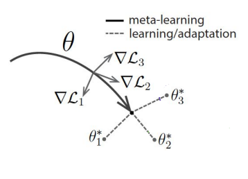
Optimization algorithm idea
The algorithm can be written as:
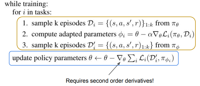
Optimization algorithm idea
Notice that \(\theta\) receives credit for providing good exploration policies.
Pros/Cons:
- Conceptually elegant.
- It is consistent (good extrapolation): It is just gradient descent.
- It is NOT as expressive: If no rewards are collected adaptation wil not change the policy, even when this data gives information about states to avoid.
- Complex, requires a lot of samples.
More on:
-
Papers on meta-policy gradient estimators: Model-Agnostic Meta-Learning for Fast Adaptation of Deep Networks, DiCE: The Infinitely Differentiable Monte-Carlo Estimator, ProMP: Proximal Meta-Policy Search.
-
Papers on improving exploration: Meta-Reinforcement Learning of Structured Exploration Strategies, Some Considerations on Learning to Explore via Meta-Reinforcement Learning
-
Hybrid algorithms: Evolved Policy Gradients, MetaLearning by the Baldwin Effect
Meta-RL as an POMDP
Idea: Meta-RL corresponds to regular RL but on a POMDP. In this case, we would define the policy to work on the observation-space instead of the state-space: \(\pi_\theta (a \mid o)\). This requires either:
- Explicit state estimation: i.e. \(p(s_t \mid o_{1:t})\)
- Use policies which have memory: i.e. learning \(\pi_\theta (a \mid s, z)\), where \(z\) encapsulates the information a policy needs to solve the current task (as we saw in RNN-based Meta-RL)
Let’s now focus on explicit state estimation techniques.
Explicit State Estimation
Given some trajectory, we want to estimate an underlying state describing it: \(p(z_t \mid s_{1:t}, a_{1:t}, r_{1:t})\). Then, we can explore via posterior sampling with some latent context:
Repeat:
- Sample \(z \sim \hat p (z_t \mid s_{1:t}, a_{1:t}, r_{1:t})\) (One can use a variational approach)
- Act according to \(\pi_\theta (a \mid s, z)\) to collect more data
Which means we are finding the parameters \(\theta, \phi\) (policy and inference network) that satisfy:
\begin{equation} (\theta, \phi) = \arg \max_{\theta, \phi} \frac{1}{N} \sum_i E_{z \sim q_\phi, \tau \sim \pi_\theta} \left[ R_i(\tau) - D_{KL} (q(z \mid …) \Vert p(z))\right] \end{equation}
Where \(p(z)\) is the prior we picked for the \(z\) distribution. \(\hat p (z_t \mid s_{1:t}, a_{1:t}, r_{1:t})\) can be encoded by any architecture but one shown to present good results is Probabilistic Embeddings for Actor-Critic RL (PEARL) presented in Efficient Off-Policy Meta-Reinforcement Learning via Probabilistic Context Variables, which is order-agnostic by exploiting the Markov Property.
Problem: This procedure does not resolve in information gathering actions. When sampling, you sample from your hypothesis on what the task might be and them attempt to solve that task, but the thing you do to determine what task is, might be different from what you would do for that particular task. Nevertheless, in practice, it works pretty good.
Pros/Cons:
- Simple and effective exploration via posterior sampling.
- Elegant reduction to solving special POMDP.
- It is consistent (good extrapolation): It is just gradient descent.
- Vulnerable to meta-overfitting
- Challenging to optimize in practice.
Model-Based Meta-RL
Remember standard model-based RL:
Repeat:
- Collect data \(\mathcal{B}\)
- Use data \(\mathcal{B}\) to get \(\hat p (s_{t+1} \mid s_t, a)\)
- Use \(\hat p (s_{t+1} \mid s_t, a)\) to plan actions.
Pros/Cons:
- Requires much less data than model-free.
- Can adapt extremely quickly.
- This is non-adaptive: If something changes in the environment this algorithm will not be able to respond!
Adaptive Model-Based Meta-RL
Let, \(d_\theta (s, a) \rightarrow s^\prime\) the function which returns the next expected state given a state-action pair \((s, a)\).
Repeat:
- Take 1 step, get \(\{ s, a, s^\prime \}\)
- Update model parameters according to the seen changes: \(\theta \leftarrow \theta - \alpha \nabla_\theta \Vert d_\theta (s, a) - s^\prime \Vert^2\)
- Use \(d_\theta\) to select action
This way we are accounting for dynamic changes in the environment. In fact, the field of adaptive control is concerned with this problem, using simple linear models instead of neural nets.
For this to work though, you need to train considering these possible changes in dynamics. The way it is done is by constructing a meta-training dataset:
\begin{equation} \mathcal{D}_{\text{meta-train}} = { (\mathcal{D}^{train}_1, \mathcal{D}^{test}_1), …, \mathcal{D}^{train}_n, \mathcal{D}^{test}_n)} \end{equation}
Where each dataset is a sampled subsequence of a past experience trajectory (assuming they have different dynamics).
\begin{equation} \mathcal{D}^{train}_i = { ((s^i_1, a^i_1), s^{\prime, i}_1) , …, ((s^i_k, a^i_k), s^{\prime, i}_k) } \end{equation}
\begin{equation} \mathcal{D}^{test}_i = { ((s^i_1, a^i_1), s^{\prime, i}_1) , …, ((s^i_k, a^i_l), s^{\prime, i}_l) } \end{equation}
Intuitively, given a trajectory, we would sample the dataset as so:
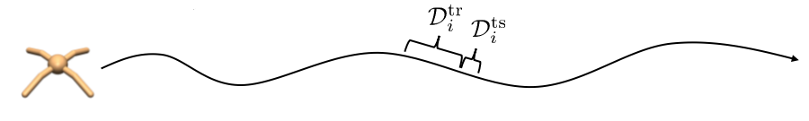
Illustration of datasets in adaptive model-based meta-rl.
More on this idea on: Learning to Adapt in Dynamic, Real-World Environments Through Meta-Reinforcement Learning
Discussion
Now that we know a bit more on Meta-RL research, it would be interesting to see how related it is to how biological beings learn. Biological beings seemingly present multiple learning behaviors:
- Highly efficient but (apparently) model-free RL
- Episodic recall
- Model-based RL
- Causal inference
Are all of these really separate brain “algorithms” or could they be emergent phenomena resulting from some meta-RL algorithm? The following papers discuss this:
- Been There, Done That: Meta-Learning with Episodic Recall
- Prefrontal cortex as a meta-reinforcement learning system
- Causal Reasoning from Meta-Reinforcement Learning
Cited as:
@article{campusai2021mrl,
title = "Meta-Reinforcement Learning Basics",
author = "Canal, Oleguer",
journal = "https://campusai.github.io/",
year = "2021",
url = "https://campusai.github.io/rl/meta-rl"
}