CampusAI

In this post we will first understand what are the main challenges of working with high-dim data. Later, we will go through the most famous approaches to reduce data dimensionality while preserving as much information as possible.

The curse of dimensionality

The curse of dimensionality refers to the set of problems which arise when working in high-dim spaces. These include:

Space volume grows exponentially with the number of dimensions. Thus available data becomes very sparse. The volume is very large compared to the number of datapoints.
Often in high-dim spaces many dimensions are irrelevant for the considered task.
High-dim data visualization is difficult, making it hard to understand.
Geometry in high-dim spaces is not intuitive.

Before we jump into the most used algorithms lets take refresh our memory on matrix SVD decomposition (as most of them rely on it).

Space volume grows exponentially?

1-d: Imagine your data lies in a line of 10 units of length. The “volume” of space is $10^1$.
2-d: If the data is instead in a plane of 10 units by side. The “volume” of space is $10^2$.

In 3-d the volume would be $10^3$… The volume is growing exponentially with the number of dimensions as data-points become more isolated.

SVD: Singular Value Decomposition

Matrix decomposition is expressing a matrix as a product of other matrices which certify some conditions.

Some famous decompositions not presented in this post are: LU Decomposition, Cholesky Decomposition, Polar Decomposition

Before explaining the idea behind SVD dimensionality reduction, lets take a look at the SVD theorem:

SVD Theorem: Any matrix $A \in \mathbb{R}^{m \times n}$ can be factorized into:

\begin{equation} A = U \Sigma V^T \end{equation}

Where:

$U \in \mathbb{R}^{m \times m}$ is an orthogonal matrix (its cols form an orthonormal basis).

$\Sigma \in \mathbb{R}^{m \times n}$ is diagonal with elements: $\space \sigma_1 \geq \sigma_2 \ge ... \ge \sigma_k \ge 0$. Where $k = min\{m, n\}$.

$V \in \mathbb{R}^{n \times n}$ is an orthogonal matrix (its cols form an orthonormal basis).

Geometrically SVD theorem is telling us that any linear transformation between vector spaces can be achieved by a rotation ($V$) in the src space, a dilation + projection ($\Sigma$) into the final space and another rotation ($U$) in the final space.

Naming goes:

Singular values: $\{\sigma_i \}_i$
Right singular vectors: Columns of $V$
Left singular vectors: Columns of $U$

So, lets see how we can take advantage of this type of matrix decomposition:

Notice that:

$A v_i = \sigma_i u_i$.
$A^T u_i = \sigma_i v_i$.

Theorem:

Let $A = U \Sigma V^T$ be the SVD of $A$

Let $U_k = (u_1, ..., u_k)$ be the first k cols of $U$

Let $V_k = (v_1, ..., v_k)$ be the first k cols of $V$

Let $\Sigma_k = (\sigma_1, ..., \sigma_k)$ be the k largest singular values

Then: \begin{equation} A_k = U_k \Sigma_k V_k^T \end{equation}

Is the closest projection of $A$ into the space of matrices of rank-k w.r.t the spectral norm, and its distance to $A$ is $\sigma_{k+1}$: \begin{equation} \min_{B s.t. rank(B) \le k} \Vert A - B \Vert_2 = \Vert A - A_k\Vert_2 = \sigma_{k+1} \end{equation}

This is all SVD dim-reduction does: Keep the k biggest singular values of the SVD and discard the rest. We are approximating $A$ by only using the information of the gray areas of the SVD in this image:

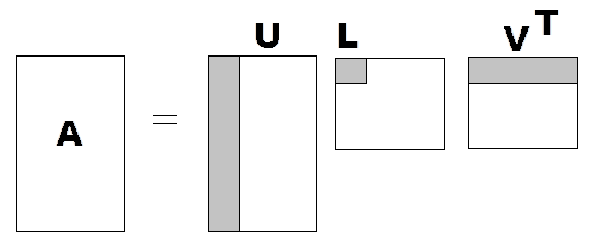
Figure 1: Matrix approximation by selecting the first k singular values (gray area). Instead of representing $A$ by all its $m \times n$ values we can approximate it with $m \times k + k + k \times n \ll m \times n$. Figure from http://ezcodesample.com/.

Interpretation

We now have a matrix $A_k \simeq A$ which can be stored using way less information as fig. 1 shows. But, what does this mean? Lets first think of $A \in \mathbb{R}^{n \times m}$ as a linear map between two vector spaces:

\begin{equation} A_{n \times m}: \mathcal{V} \subseteq \mathbb{R}^m \rightarrow \mathcal{U} \subseteq \mathbb{R}^n \end{equation}

In this case, SVD finds an orthonormal base $\mathcal{B}_\mathcal{V} = \{v_1, ... v_m\}$ in $\mathcal{V}$ and another one $\mathcal{B}_\mathcal{U} = \{u_1, ... u_n\}$ in $\mathcal{U}$ such that between those bases $A$ is diagonal ($\Sigma$).

For instance: If $A \in \mathbb{R}^{3 \times 2}$, SVD pairs: $v_1 \rightarrow u_1, v_2 \rightarrow u_2$. Such that EVERY point $p = (p_1 , p_2)_{\mathcal{B}_\mathcal{V}}$ gets mapped to $q = (\sigma_1 \cdot p_1 , \sigma_2 \cdot p_2, 0)_{\mathcal{B}_\mathcal{U}}$:

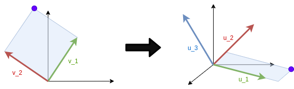
Figure 2: Representation of A mapping SVD. Left singular vectors in the 2-d space are mapped to right singular vectors in 3-d space. In this case $\sigma_1 \gg \sigma_2$. Figure by CampusAI.

As we saw, SVD matrix approximation ignores the dimensions where the dilation is factor ($\sigma_i$) is close to $0$ In the image, $\sigma_2$ is much smaller than $\sigma_1$, if we remove the second dimension our mapping approximation will lie in a line. The purple point will then be on the $u_1$ direction.

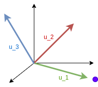
Figure 3: Effect of removing the second dimension. Notice that the purple point is relatively close to the `real` position. Figure by CampusAI.

In general:

If $m \le n$, $A$ maps space $\mathcal{V}$ into a subspace of dimension m in $\mathcal{U}$.

In particular, the one which $A$ presents a larger dilation.

If $m \ge n$, $A$ fills the whole destination space $\mathcal{U}$. Keeping only the first $k$ dimensions will project into the $k$-dim subspace of larger dilation.

Matrix as a transformation or matrix as data?

You now might think something like: Wait, what if my matrix is not a transformation but just a table with data?

Is it really “just a table” though? The 2006 Netflix prize is a great example to see the connection between matrices as data tables and matrices as transformations. Netflix provided a dataset of users vs movie ratings as:

I oversimplified this section for readers to just get the general idea, if interested in this topic read this great post on SVD interpretation.

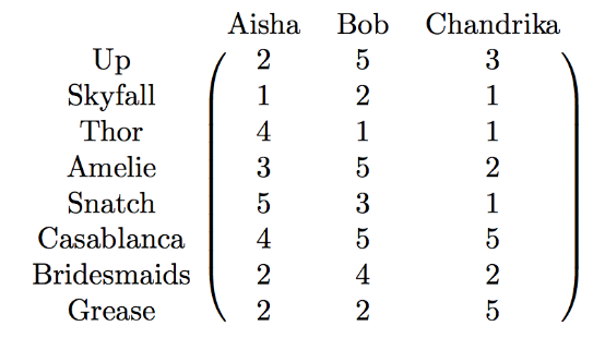
Figure 4: Movie ratings examples. Figure from jeremykun.com.

The prize was 1.000.000$ for team which achieved at least 10% less RMSE error than Cinematch (Netflix’s recommender system used at that time). And yeah, you guessed it: the winners used SVD (otherwise I wouldn’t be talking about this duh).

So, where is the connection? We can also understand this data matrix as a transformation from the user-space ($\mathcal{V}$) to the movie-space ($\mathcal{U}$): If I’m 70% like Aisha 25% like Bob and 5% like Chandrika my movie ratings will be a linear combination of Aisha’s, Bob’s and Chandrika weighted by my similarity to each one of them. If do the dot product of the matrix to my similarity vector $(0.7, 0.25, 0.05)$ I get my most likely movie ratings (the matrix is now a transformation).

SVD finds a base in the user-space which is “aligned” to a base in the movie-space. Each right singular vector $v_i$ encodes the person archetype who “just cares” for an associated archetype movie represented by a left singular vector $u_i$ with a strength of $\sigma_i$.

We can express each person as a combination of archetype people, which will like their associated archetype movies. Moreover, we can pick $k$ to have as many archetypes as we want to cluster people’s preferences.

For instance, you can think of an archetype person $v_i$ your grandad and an associated archetype movie $u_i$ westerns.

Relation to Eigen Decomposition

Eigen decomposition (aka spectral decomposition) is the decomposition of a square and diagonizable matrix into eigenvectors and eigenvalues:

\begin{equation} A = Q \Lambda Q^{-1} \end{equation}

Where $Q = (v_1, ... v_n)$ is an orthogonal matrix composed by the eigenvectors $\{v_i\}_i$ and $\Lambda$ is diagonal with the eigenvalues $\{\lambda_i\}_i$. Remember that an eigenvalue, eigenvector pair satisfy: $A v_i = \lambda_i v_i$, they represent the directions in which the transformation is a simple scaling. For visual interpretation I recommend checking out this video.

If you take a look on the SVG theorem proof you’ll see SVG is based on the Eigen decomposition of $A^T A$. In essence:

$\{\sigma_i \}_i$: singular values of $A$ are: $\{ \sqrt{\lambda_i} \}_i$ square root of eigenvalues of $A^T A$.
Right singular vectors of $A$ (columns of $V$) are eigenvectors of $A^T A$.
Left singular vectors of $A$ (columns of $U$) are eigenvectors of $A A^T$.

If $A \in \mathbb{R}^{n \times n}$ is symmetric with non-negative eigenvalues, then eigenvalues and singular values coincide.

To see how these ideas are applied to different dim reduction problems, check out our following post on the main Dim reduction algorithms.

Dimensionality reduction: Algebraic Background

The curse of dimensionality

SVD: Singular Value Decomposition

Interpretation

Matrix as a transformation or matrix as data?

Relation to Eigen Decomposition