Dimensionality reduction: Algorithms
I highly recommend to read the previous post: Dim reduction basics to get familiar with SVD. So, how can we cope with high-dim data?
-
Quantify relevance of dimensions and (possibly) eliminate some. This is commonly used in supervised learning, where we pay more attention to the variables which are more highly correlated to the target.
-
Explore correlation between dimensions. Often a set of dimensions can be explained by a single phenomena which can be explained by a single latent dimension.
PCA: Principal Component Analysis
Consider a dataset \(\mathcal{D}\) of \(n\) points in a high-dim space \(x_i \in \mathbb{R}^d\). In a matrix form: \(X \in \mathbb{R}^{d \times n}\).
Assumptions:
- For each data-point \(x_i \in \mathcal{D}\) there exists a latent point in a lower-dim space \(z_i \in \mathbb{R}^k\) which generates \(x_i\).
- There exists a linear mapping (
decoder) \(W \in \mathbb{R}^{d \times k}\) s.t. \(z_i = W^T x_i \space \forall (z_i, x_i)\) - \(W\) has orthonormal columns (i.e. \(W^T W = I_{k \times k}\), notice that usually \(W W^T \neq I_{d \times d}\)).
PCA works on CENTERED data (looks for linear projections). You need to substract the mean.
So far we have a decoder:
\begin{equation} \textrm{dec}: \mathcal{Z} \subseteq \mathbb{R}^k \rightarrow \mathcal{X} \subseteq \mathbb{R}^d \mid \textrm{dec(z)} = W z \end{equation}
And an encoder:
\begin{equation} \textrm{enc}: \mathcal{X} \subseteq \mathbb{R}^d \rightarrow \mathcal{Z} \subseteq \mathbb{R}^k \mid \textrm{enc(x)} = W^T x \end{equation}
Optimization criteria: PCA aims to minimize the MSE between original data and the reconstruction: \(\min E_x \left[ \Vert x - dec(enc(x)) \Vert_2^2 \right]\), which is:
\begin{equation} \min_W E_x \left[ \Vert x - W W^T x \Vert_2^2 \right] = \min_W \underbrace{E_x \left[ x^T x \right]}_{\textrm{constant wrt } W} - E_x \left[ x^T W W^T x \right] \end{equation}
Therefore we aim to minimize:
\begin{equation} \min_W - E_x \left[ x^T W W^T x \right] = \max_W E_x \left[ x^T W W^T x \right] = \max_W \frac{1}{n} \sum_i^n x_i^T W W^T x_i = \max_W \frac{1}{n} \text{tr} \left( X^T W W^T X \right) \end{equation}
If we consider the SVD of \(X\):
\begin{equation} \text{tr} \left( X^T W W^T X \right) = \text{tr} \left( V \Sigma U^T W W^T U \Sigma V^T \right) \end{equation}
Which can be shown that the maximum is achieved by taking \(W = U_k\). I.e. to project the data using the first k singular vectors of X. As you can see, SVD gives a nice connection between explained variance of the data and reconstruction error through singular values:
- First k ppal components variance: \(V_W = \sum_{i=1}^k \sigma_i^2\)
- Reconstruction error: \(E_W = \sum_{i=k+1}^d \sigma_i^2\)
We can use this idea to select an appropriate k to explain a certain percentage of data. For instance, if we want our encoding to explain at least 85% of the data variance:
\begin{equation} \min_k \mid \frac{V_W}{V_X} = \frac{\sum_{i=1}^k \sigma_i^2}{\sum_{i=d}^k \sigma_i^2} \ge 0.85 \end{equation}
Interpretation
PCA focusses on what makes the data more different from each other: it keeps the directions with higher variance. Image you construct the data matrix \(X_{d \times n}\) where each column is a data-point. If you know how similar you are to a subset of datapoints you can guess your position (if you multiply similarity by this matrix you get the position in the $d$-dimensional space):
\begin{equation} \begin{bmatrix} \vdots & \space & \vdots \newline x_1 & \cdots & x_n \newline \vdots & \space & \vdots \end{bmatrix} \cdot \underbrace{ \begin{bmatrix} 0.1 \newline \vdots \newline 0.03 \end{bmatrix}} _{\textrm{Similarity to each datapoint}} \end{equation}
As we said before, left singular vectors of SVD \((u_1, ..., u_k)\) give the directions in final space in which there is larger dilation sorted by magnitude: The directions in which there is a larger spread of data (thus being similar to a point is more representative). Therefore, if most data-points (vectors) lay in a line the largest elongation will be along that direction. In the picture, \(A \in \mathbb{R}^{2 \times n}: \mathbb{R}^n \rightarrow \mathbb{R}^2\) has larger elongation along the pink marks axis.
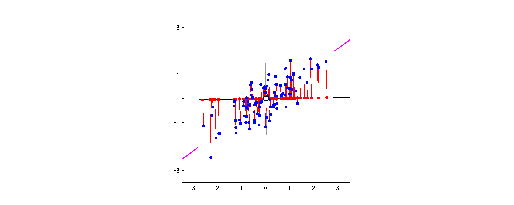
Figure 5: 2D points linear projection into 1D space. Notice that the axis of higher variance (first left singular vector) provides the most informative projection. Figure from https://builtin.com/ (Zakaria Jaadi)
If you apply PCA, you dont need to work with all datapoints, but just keep the most representative directions (singular vectors) and their weight (singular values).
I highly recommend this video for PCA interpretation.
RECAP
PCA finds the linear projection into the subspace of dimension $k$ whith lowest MSE reconstruction. This space is spawned by the directions of highest variance in the data: k-largest singular-value vectors of SVD decomposition of data matrix.
Kernel-PCA
It is often the case that for some dataset, a linear projection is not enough. Consider this example of a 2D surface embedded into a 3D space. No matter how you orient the projection plane (if \(k=2\)), the projection will not be good:
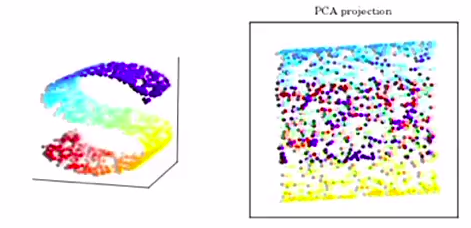
Figure 6: PCA of s-shaped surface into a 2D space. Figure from David Thompon Carltech kernel-PCA lecture.
The main idea of kernel-PCA is to non-linearly project the data into a higher-dimensional space so that the data becomes easier to project from there. Given a non-linear function \(\phi\): we minimize the following objective:
\begin{equation} \min E_x \left[ \Vert \phi(x) - W W^T \phi(x) \Vert_2^2 \right] \end{equation}
Same as before, we would do SVD of \(\phi(X) \phi(X)^T\).
Kernel Trick
Usually its not needed to explicitly compute the (even higher-dimensional) \(\phi(X)\). It is enough to compute the pairwise dot product between all pairs of points: \(k(x_i, x_j)\). If smartly choosing \(\phi\) this dot product can be found from the low-dim space, making the computation much more efficient. This technique is known as “the kernel trick”.
MDS: Multi-Dimensional Scaling
Classic MDS
Classical MDS (aka PCoA: Principal Coordinate Analysis) solves the following input-output problem:
- Input: Pair-wise euclidean distance matrix between points in high-dim space.
- Output: Point coordinates in low-dim space (aka coordinate matrix).
More formally: Given a set of pair-wise euclidean distances \(d_{ij}\) between point \(i\) and point \(j\), Classical MDS finds the latent points \(z_1, ..., z_n\) which minimize the following metric:
\begin{equation} Stress_p (z_1, …, z_n) = \left( \sum_{i < j}^n \left( \Vert z_i - z_j \Vert - d_{ij} \right)^2 \right)^{\frac{1}{2}} \end{equation}
Same as in PCA, we need to center the data. We do this by making the distance matrix columns and rows sum to zero by multiplying it on both sides by a centering matrix. This is known as the double centering trick. Once we have this matrix, the procedure is analogous to the one from PCA. In summary:
Classical MDS algorithm:
- Get squared distance matrix \(D := \left[ d_{ij}^2 \right]\)
- Double-center the distance matrix: \(B := -\frac{1}{2} J D J\), where \(J\) is a centering matrix.
- Get spectral decomposition of \(B\) and select k-highest eigenvals: \(\Lambda := diag(\lambda_1, ..., \lambda_k)\), \(E_k := [v_1 \cdots v_k]\)
- The k-dim data is then: \(Z^T = E_k \Lambda^{\frac{1}{2}}\)
MDS can be seen as a dim-reduction technique since it can produce embeddings which preserve the structure of the data.
Obviously, the solutions given by MDS are not unique. Translations, rotations, and mirrorings do not alter the distances.
Model-checking is usually done plotting a scatter plot of original vs latent distances. You can easily detect biases if the datapoints do not lie in the diagonal.
MDS vs PCA: PCA and MDS solve different problems using the same idea.
- PCA aims to find the subspace of larger variance by using the data covariance matrix (a measure of correlation between points)
- MDS applies the same algorithm to find points in a lower-dim space which are distanced equally as the points in the high-dim space.
- With MDS you don’t need to know the actual feature values, just the distance or (dis)similarity between the points.
This has been exploited to map complex elements using the averages of qualitative distances given by humans.
mMDS (metric-MDS)
Metric MDS is a generalization of classical MDS. Remember that classical MDS assumes the provided distances are euclidean \((L^2)\) which can be very limiting. Metric MDS generalizes Classical MDS to use any other distance.
\begin{equation} Stress_p (z_1, …, z_n) = \left( \sum_{i < j}^n w_{ij} \left( \Vert z_i - z_j \Vert - d_{ij} \right)^2 \right)^{\frac{1}{2}} \end{equation}
Where \(w_{ij}\) is a weight given to that distance difference. A common choice is \(w_{ij} = \frac{1}{d_{ij}}\) (aka Sammon’s nonlinear mapping). In this case we “care” more about close things and less about far things.
mMDS vs MDS:
- Working with any distance function provides more expressivenes.
- Greater generality comes at the cost of no closed-form solution. Need to use some generic optimizer (e.g. gradient descent).
nmMDS (non-metric-MDS)
Non-metric MDS is yet another generalization. for when instead of having distance information you have ordinal information of the data. This is: you only know some ordering (or ranking) of it instead of some quantitative distance. Given the pairwise ordinal proximities \(\delta_{ij}\) between a set of elements, we are trying to minimize:
\begin{equation} E_{nmMDS} (z_1, …, z_n) = \left( \sum_{i < j}^n w_{ij} \left( \Vert z_i - z_j \Vert - f(\delta_{ij}) \right)^2 \right)^{\frac{1}{2}} \end{equation}
Where \(f\) is a monotone transformation of proximities.
Isomap
Idea: Euclidean distance in the original space might be a poor measure of dissimilarity between points. Instead the geodesic distance might be more informative.
Problem: Computing the geodessic distance between any two points without knowing the manifold is too hard.
Solution: For close points: Euclidean \(\simeq\) Geodessic. We can approximate long distances by doing a sequence of “short hops”. We can model this with a graph.
The main algorithm then becomes:
Classical MDS algorithm:
- Given dataset \(\mathcal{D} = \{x_i\}_i\). Compute Euclidean distances among the points \(d_{ij}\).
- Construct a graph where each vertex is a point and its connected to the p nearest neighbors.
- For each pair of points (\(x_i\), \(x_j\)) compute the shortest path distance (using the graph) \(\delta_{ij}\).
- Use MDS on these \(\delta_{ij}\) to compute the low-dim embedding \(\{z_i\}_i\).
Disadvantages:
- Sensitive to noise.
- Sensitive to the number of neighbours.
- If the graph is disconnected, the algorithm will fail.
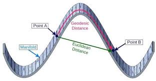
Euclidean vs Geodessic distances. Image from A. Yamin et al., Comparison Of Brain Connectomes Using Geodesic Distance On Manifold: A Twins Study
Autoencoders
Another recently popular non-linear dim-reduction technique is to use ANN-based autoencoders. In a nutshell: you train a sandclock shaped neural network to reconstruct your data forcing the middle layer to learn a compressed representation of it. The objective function (loss) optimized is essentially the same as the ones we’ve seen so far. For instance, if we want to minimize the MSE between each input and its reconstruction:
\begin{equation} \min_{\phi} \Vert x - dec_\phi(enc_\phi(x)) \Vert_2^2 \end{equation}
Where enc and dec are ANNs which can be trained with gradient descend.
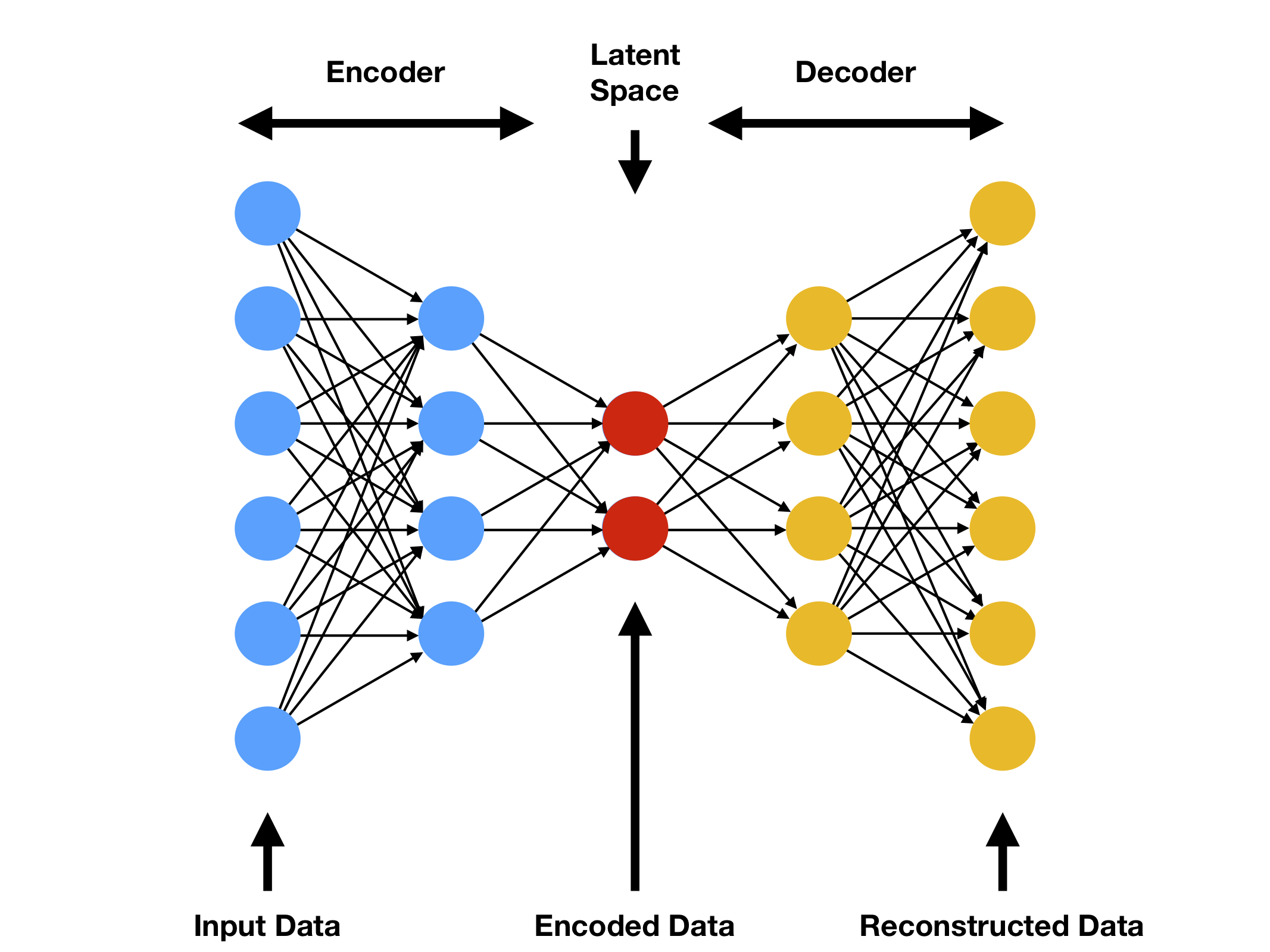
Figure 7: Standard autoencoder architecture. First half of the neural networks works as a data compression encoder, second half reconstructs the input to its decompressed form. Figure from compthree blog
Note the similarity with PCA. PCA is a special case where the ANNs only have 1 dense layer without activation function and share the same parameters to encode and decode (transposed).
We talk more about autoencoders (and their more interesting evolution: variational-autoencoders VAEs) in this Latent Variable Models post.