Recommender Systems
Recommender system address the following question: Given a set of users, items, and their past interactions, how can we recommend the best item for each user?
These past interactions are usually stored in a matrix called the user-item interaction matrix. It can contain ratings of movies, likes/dislikes of videos, song reproductions…
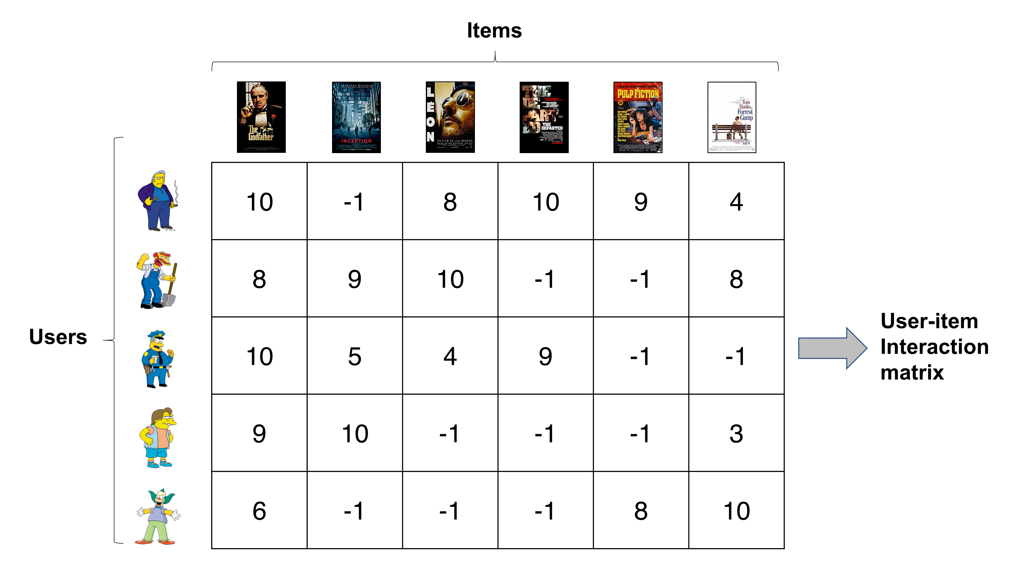
Each row contains a different user rating of a movie (cols). (Image from buomsoo-kim.github.io/)
In our day-to-day life, we are constantly interacting with recommender systems: YouTube recommends us new videos, Amazon shows us items of interest, Spotify proposes playlists…
Collaborative filtering methods
Collaborative filtering methods are solely based on the interaction between users and items. Thus (unlike content-based methods) they do not process features of the items.
Pros/Cons:
- Require no information about users or items.
- They improve over time: more interactions \(\rightarrow\) better recommendations.
- Cold-start problem: Cannot make predictions to new users (no past interactions available).
Cold-start problem can be addressed in multiple ways:
- Random strategy: Recommending random items to new users (or new items to random users).
- Maximum expectation strategy: Recommending most popular items to new users.
- Exploration strategy: Recommending a set of various items to new users (or a new item to a set of various users).
- Not using a collaborative method for new-coming users.
Memory-based
Memory-based collaborative filtering usually uses kNN (k-nearest neighbor) search from the information on the user-item interaction matrix.
Pros/Cons: Same as k-NN algorithm in general:
- Low bias.
- High variance.
- Bad scalability: kNN search can be slow if dealing with millions of users and items (need to use approximate kNN methods).
- No model \(\rightarrow\) lack of regularization: It is hard to avoid recommending only either popular items or items extremly similar to the ones already consumed.
User-User
Imagine we want to recommend something to a given user \(x\). These method would find the most similar users and recommend something these users enjoyed that hasn’t been consumed by \(x\). This similarity is computed using some distance metric between each user’s row in the user-item interaction matrix, accounting for the un-interacted items.
Similarity between users is often evaluated using the centered cosine similarity (aka Pearson’s coefficient)
We can get an estimation of the rating a user \(x\) will give to item \(i\) as:
\begin{equation} r_{x,i} = \frac{\sum_{y \in \text{SIM}(x)} s_{xy} r_{yi}}{\sum_{y \in \text{SIM}(x)} s_{xy}} \end{equation}
Where:
- \(\text{SIM}(x)\) represents the subset of users which are similar to \(x\).
- \(s_{xy}\) represents the similarity between user \(x\) and user \(y\).
Item-Item
Item-item methods use the same idea but from the perspective of items instead of users. When recommending something, instead of looking at similar users, we can look at similar items to those already liked by the user and recommend these.
The estimated rating would then be:
\begin{equation} r_{x,i} = \frac{\sum_{j \in \text{SIM}(i)} s_{ij} r_{xj}}{\sum_{j \in \text{SIM}(i)} s_{xj}} \end{equation}
Where:
- \(\text{SIM}(i)\) represents the subset of items similar to item \(i\).
- \(s_{ij}\) represents the similarity between item \(i\) and item \(j\).
Other ideas:
Depending on the nature of the service provided one can better exploit the data and get the similarity between items by alternative means. For instance, Spotify users organize songs in playlists: This aggregations can be understood in different ways:
- Framing the problem as frequent itemset detection: Songs are items and playlists are baskets. We can then run the A Priori algorithm to detect songs that are frequently together in lists.
- Looking from a NLP perspective, we can think of song ids as words and playlists as documents. Then we can train something similar to word2vec (or any other word embedding algorithm) and obtain a projection of song_ids into a latent space where similar songs will be close to each other.
word2vec is essentially implemented as an autoencoder that embeds words into a latent space considering its syntactic similarity.
Comparison with user-user:
- Item-item works better than user-user, as human’s complexity tends to be higher than item’s one.
- Item-item has less variance: A lot of users have interacted with an item but each user interacts with few items, so item similarities are less sensitive.
- Item-item has higher bias: Item similarity is assessed from very different users, so the method is less personalized.
Model-based
Pros/Cons:
- Smaller variance than memory-based methods (less dependent on data).
- Higher bias than memory-based methods (assumptions are made when choosing a model).
Matrix factorization
The idea is to factorize the huge (and very sparse) user-item interaction matrix \(M \in \mathbb{R}^{n \times m}\) into two small and dense matrices:
- The user-factor matrix \(Q \in \mathbb{R}^{n\times l}\): Each row contains the projection of a user into the latent space.
- The factor-item matrix \(P \in \mathbb{R}^{m\times l}\): Each row contains the projection of an item into the latent space.
\begin{equation} M = Q P^T \end{equation}
In essence, we learn a (linear) model to represent both users and items in a low-dimensional space (of \(l\) dimensions). The low-dim features of a user will match those of the movies it enjoys.
A possible factorization would be using SVD (check out our dimensionality reduction post). However SVD is very expensive (considering how big the user-item interaction matrix is) and does not account for all the missing information. Alternatively, we can see it as an optimization problem, where we look for tha matrices which give the best reconstruction:
\begin{equation} P, Q = \arg \min_{P, Q} \sum_{(i, j) \in \text{RATINGS}} \left[ P_i Q_j^T - M_{ij} \right]^2 + \underbrace{\lambda_p \Vert P_i \Vert^2 + \lambda_q \Vert Q_j \Vert^2}_{regularization} \end{equation}
The regularization ensures we assign \(0\) to the unknown interactions.
We can then find \(P, Q\) running gradient descent on that loss. With the advantage that we can train with batches of users and items independently.
Once we have the matrices factorized we can either:
- Predict user \(i\) rating on item \(j\) by doing the dot product: \(r_{ij} \simeq P_i Q_j^T\).
- Run memory-based algorithms (user-user, item-item) on this much smaller and dense vectors.
More generally, we can estimate the rating given by users by fancier operation than dot product such as an ANN \(f_\phi\):
\begin{equation} P, Q, \phi = \arg \min_{P, Q, \phi} \sum_{(i, j) \in \text{RATINGS}} \left[ f_\phi (P_i, Q_j) - M_{ij} \right]^2 + \underbrace{\lambda_p \Vert P_i \Vert^2 + \lambda_q \Vert Q_j \Vert^2}_{regularization} \end{equation}
Content-based methods
Content-based methods process features of the items and/or users to find the best recommendations. In essence, they try to build a model that explains the observed user-item interactions. Once trained, we can run inference by inputing user features. The model will output a set of matching items.
Pros/Cons:
- Suffers far less from cold-start problems.
- Smaller variance than collaborative methods.
- Higher bias than collaborative methods (assumptions are made when choosing features and model).
- Harder interpretation.
In a song recommender system:
- User features can be: age, sex…
- Item features can be: group, genre, year…
Types:
- User-centered: For each user we train a model using item features. Same as user-user methods, it is much more personalized as it is only trained on items the user has interacted with. However, it is less robust as each user hasn’t interacted with a lot of items.
- Item-centered: Train a model for each item which once inptued user features, outputs an estimated rating. Same as item-item methods, it is more robust (less variance) but less personalized (more bias), as some users with similar features can have dissimilar taste.
- Combinations: We can also consider models that process both user features and item features and guess some affinity. After the success of collaborative filtering and with the rise of ANNs, this approach has been very successful. However, industry hit a plateau where it was hard to achieve a significant advantage until RL approaches came along.
If looking for simple models we can use Naive Bayes or Logistic regression for classification scenarios and linear regression for regression tasks. Or we can learn more complex models using ANNs.
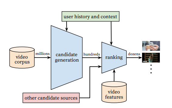
Funnel structure of youtube recommender system. First screening is done with basic SQL queries, the second one using an ANN architecture. (Image from Deep Neural Networks for YouTube Recommendations)
While these item features can be hand-crafted by humans, it is interesting to study how they can be automatically extracted using ML techniques. For instance, Spotify can get characteristics of a song by analyzing its audio file and learning a model that relates songs by these signatures. This can be very helpful to solve the cold-start problem as it can be trained in a supervised fashion with past songs whose similarity is known using collaborative filtering techniques.
Item-centered answers the question: What is the probability of each user to like this item?, while user-centered methods answer the question: What is the probability of each item being liked by this user?.
It is also interesting to note that usually asking for information to new users is much harder than obtaining item information. Thus, item features tend to be much better than user features.
Reinforcement Learning approach
Collaborative filtering and content-based methods mainly belong to the supervised learning paradigm. SL presents some limitations to solve the recommendation problem:
- It doesn’t consider the selection bias the recommender itself introduces.
- Myopic recommendation: Recommender doesn’t consider long-term user retention, only provides content immediately interesting to the user without considering exploration.
Framing the problem as an interactive system where the recommender presents some content and users review this content might be better. However, it still presents some challenges:
- Large action space: Millions of items.
- Expensive exploration: Space is very big.
- Needs to be off-policy: Most of the data comes from different policies (users). Can be solved using importance sampling.
- Partial observability: Only part of the state can be inferred.
- Noisy reward.
RL problem setup:
- Agent: Candidate generator.
- States: User interest profile, context.
- Actions: Nominate from a catalog od millions of videos.
- Reward: User satisfaction and long-term engagement.
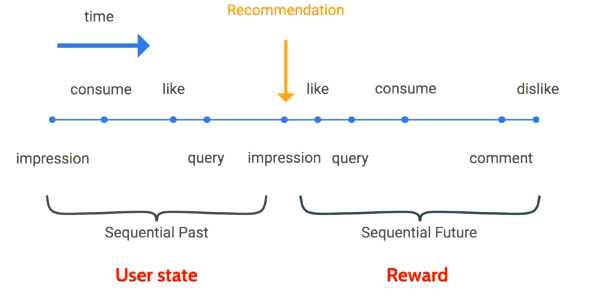
Visualization of RL setup. They used a policy gradient approach to learn a policy. (Image from Deep Neural Networks for YouTube Recommendations)
Evaluating Recommender Systems
How do you know if your model is any good? Notice that users will not like a model that proposes things which are too similar to what they already know, there also needs to be some exploration. This idea is captured by the serendipity metric: the diversity of the recommendations (how close are all recommendations between themselves).
- Low serendipity \(\rightarrow\) all recommended items are very similar, which means our recommender system does not bring enough diversity (aka it creates a information confinement area)
- High serendipity \(\rightarrow\) recommended items are very different, meaning that the recommender system does not take the user enough into consideration.
Have you ever noticed that Netflix proposes new recommendations explaining why it things it is a good match? It has been shown that humans loose faith in the recommender system if they do not understand where the recommendations come from. Thus we also desire models with high explainability.
Offline evaluation
Before unleashing our recommender system into the wild, it is interesting to run some of these metrics. The main idea is to split the dataset into train and test sets and then analyze:
- Categorical Cross-Entropy (for instance) in classification tasks or MSE in regression tasks on the test set.
- If the result can be binarized (like/dislike), it is also interesting to analyze the confusion matrix metrics (precision, accuracy, AUC, …) associated with our prediction of the test set.
- In the case of recommender systems which do not output a value, but just a ranked list of items (such as collaborative memory-based ones), we can still check if any of the recommendations are present in a test set.
Online evaluation
When introducing changes into the model it is often tested using A/B testing techniques to compare its performance to some past version of the model and see if there is any statistically significant improvement.