Until now, we assumed we did not know the dynamics of the environment. Nevertheless, they are often known or can be learned. How should we approach the problem in those cases?
Deterministic environments:
Given a first state \(s_1\), you can build a plan \(\{a_1, ..., a_T\}\) defined by:
\begin{equation} a_1, …, a_T = \arg \max_{a_1, …, a_T} \sum_t r(s_t, a_t) \space \space \space \space s.t. \space s_{t+1} = \mathcal{T} (s_t, a_t) \end{equation}
To then simply blindly execute the actions.
Stochastic environment open-loop:
What happens if we apply this same approach in a stochastic environment? We can get a probability of a trajectory, given the sequence of actions:
\begin{equation} p_\theta(s_1, …, s_T \mid a_1, …, a_T) = p(s_1) \prod_t p(s_{t+1} \mid s_t, a_t) \end{equation}
In this case, we want to maximize the expected reward:
\begin{equation} a_1, …, a_T = \arg \max_{a_1, …, a_T} E \left[ \sum_t r(s_t, a_t) \mid a_1, …, a_T \right] \end{equation}
Problem: Planning beforehand if the environment is stochastic may result in total different trajectories as the expected one.
Stochastic environment closed-loop:
You define a policy \(\pi\) instead of a plan:
\begin{equation} \pi = \arg \max_{\pi} E_{\tau \sim p(\tau)} \left[ \sum_t r(s_t, a_t) \right] \end{equation}
Open-Loop planning
We can frame the planning as a simple optimization problem. If we write the plan \({a_1, ..., a_T}\) as a matrix \(A\), and the reward function as \(J\), we just need to solve:
\begin{equation} A = \arg \max_A J(A) \end{equation}
Stochastic optimization methods
Black-box optimization techniques.
Guess & Check (Random Search)
Algorithm:
- Sample \(A_1,..., A_N\) from some distribution \(p(A)\) (e.g. uniform)
- Choose \(A_i\) based on \(\arg \max_i J(A_i)\)
Cross-Entropy Method (CEM)
Algorithm:
- Sample \(A_1,..., A_N\) from some distribution \(p(A)\)
- Choose \(M\) highest rewarding samples results \(A^1,...,A^M\), the elites
- Re-fit \(p(A)\) to the elites \(A^1,...,A^M\).
Not a great optimizer but easy to code and easy to parallelize. Works well for low-dimension systems (dimensionality < 64) and few time-steps.
Improvements: CMA-ES, implements momentum into CEM.
Monte Carlo Tree Search (MCTS)
If frame the MDP as a tree (nodes are states and edges are actions), we could traverse it to find the value of each state and get an optimal policy. Nevertheless, the complete traversal of these trees is computationally prohibiting. Therefore, MCTS proposes taking only few steps from the root and approximating the value of the last visited states by running a simple policy from them (for small action spaces random policies work decently ok).
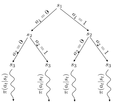
Monte Carlo shallow tree search traversal combined with simple policy to approximate state values.
Algorithm:
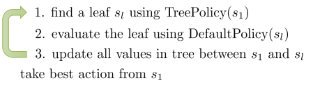
Common TreePolicy: UCT (Upper Confidence bounds applied to Trees):
- If \(s_t\) not fully expanded, choose a new \(a_t\)
- Else, choose child with best \(Score(s_t)\):
\begin{equation} Score(s_t) = \frac{Q(s_t)}{N(s_t)} + 2C\sqrt{\frac{2\log N(s_{t-1})}{N(s_{t-1})}} \end{equation}
Where \(Q(s_t)\) is the “Quality” of a state (sum of all trajectory rewards which passed through it) and \(N(s_t)\) the number of times the state has been visited. \(C\) controls how much we favour less visited nodes.
Handles better the stochastic case compared to Stochastic optimization methods. More on MCTS here. It can also substitute the human data hand-labeling in DAgger algorithm: paper
MCTS takes advantage of the model of the environment by repeatedly resetting it to the studied state.
Trajectory optimization
IDEA: Use derivatives information. To do so we’ll formulate the problem as a control one: (\(x_t\) for states, \(u_t\) for actions, \(c\) for cost) and we want to solve an optimization problem with constraints:
\begin{equation} min_{u_1,…u_T} \sum_t c(x_t, u_t) \space \space \space \space s.t. \space x_t=f(x_{t_1}, u_{t-1}) \end{equation}
Collocation method
Instead of optimizing only over actions and letting the states be a consequence of them, collocation methods optimize over both states and actions while enforcing the constrains:
\begin{equation} min_{u_1,…u_T, x_1,…,x_T} \sum_t c(x_t, u_t) \space \space \space \space s.t. \space x_t=f(x_{t_1}, u_{t-1}) \end{equation}
This usually results into a much better conditioned optimization problem than Shooting Methods (next alg.).
It is usually solved using some variant of sequential quadratic programming, locally linearly approximating the constrain and making a second-level Taylor approximation of the cost.
Shooting method
IDEA: Convert the constrained problem into an unconstrained one by substituting the constrain \(f\) and only optimizing over actions: \(\{u_1,...,u_T\}\). i.e:
\begin{equation} min_{u_1,…u_T} \sum_t c(x_1, u_1) + c(f(x_1, u_1), u_2) + … + c(f(f(…)), u_T) \end{equation}
If we had \(df, dc\), could we just do Gradient Descent (GD) at this point?
Not always.
These problems are very ill-conditioned: first actions have a huge impact on final states.
This makes easy for 1st order methods like GD get stuck, 2nd derivatives methods can help:
If open-loop, deterministic env, linear \(f\), quadratic \(c\):

Linear $f$, quadratic $c$ formulation.
Linear Quadratic Regulator (LQR): Building the second derivative matrix (Hessian) may be too expensive, LQR circumvents this issue by applying the following recursion:
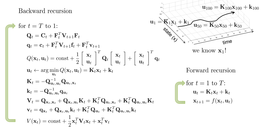
Linear LQR algorithm.
If open-loop, stochastic env, linear \(f\), quadratic \(c\):
If from Gaussian distribution: \(x_{t+1} \sim \mathcal{N} \left( F_t \begin{vmatrix} x_t,\\ u_t \end{vmatrix} + f_t, \Sigma_t\right)\), the exact same algorithm will yield the optimal result.
If closed-loop, stochastic env, linear \(f\), quadratic \(c\):
Same, using a time-varying linear controller: $K_t s_t + k_t$.
Non-linear case:
Extend LQR into iterative LQR (iLQR) or Differential Dynamic Programming (DDP).
The idea is to estimate local linear approximation of the dynamics and quadratic approximation of the cost by doing Taylor expansions. This way we can frame the problem as in simple LQR:
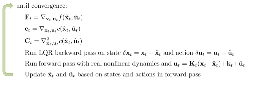
Non-linear case approximation.
This is equivalent to Newton’s minimization method (but applied to trajectory optimization). More on it in this paper.