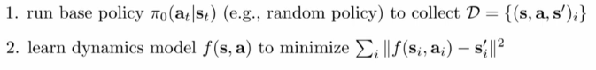
Idea: If we learn \(f(s_t, a_t) = s_{t+1}\) (or \(p(s_{t+1} \mid s_t, a_t)\) in stochastic envs.) we can apply last lecture techniques to get a policy.
Basic approaches
System identification in classical robotics:
Does it work? Yes, if we design a good base policy and we hand hand-engineer a dynamics representation of the environment (using physics knowledge) and we just fit few parameters.
Distribution mismatch problem: When we design a policy, we might be extrapolating beyond the data distribution used to learn the physics model, making results to be far off.
Solution: (Inspired by DAgger) Add samples from estimated optimal trajectory.

Problem: Blindly planning on top of an imperfect learned env. model might still result into ending up taking actions in states we did not plan to be. To improve this, we can update the plan after each step:
Model Predictive Controller (MPC)
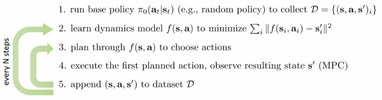
This algorithm works very decently: Replanning after each step compensates for imperfections in model and in planner. We can even plan for shorter horizons or use some very simple planner like random shooting.
Problems:
- Replanning after every step can be very expensive if we use good planners.
- Model uncertainty may lead into overestimating regions resulting into the algorithm not progressing.
Uncertainty in model-based RL
Idea: What if we exploit models being aware of their uncertainty? (similarly to Gaussian Processes)
There exist 2 types of uncertainty:
- The aleatoric (or statistical) uncertainty: Regarding the samples of the data. A good model of high aleatoric uncertainty data can have relative high entropy.
- The epistemic (or model) uncertainty: When the model is certain about the data, but we are not certain about the model (e.g. overfiting). You cannot infer that uncertainty from output entropy.
We cannot just use entropy of the ANN outcome since it is not a good measure of uncertainty. The model could be overfited and be very confident about something it is wrong about.
Estimating the posterior: \(p(\theta \mid \mathcal{D})\)
When training models, we usually only get a Maximum Likelihood Estimation (MLE) of the params: \(\arg \max_\theta \log p(\theta \mid \mathcal{D})\) (which if the priors are uniform is the same as \(\arg \max_\theta \log p(\mathcal{D} \mid \theta)\)).
Nevertheless, \(p(\theta \mid \mathcal{D})\) would tell us the real uncertainty of the model. Moreover, we could make predictions marginalizing over the parameters:
\begin{equation} p(s_{t+1} \mid s_t, a_t) = \int p(s_{t+1} \mid s_t, a_t, \theta) p(\theta \mid \mathcal{D}) d\theta \end{equation}
Bootstrap ensembling
We can achieve a rough approximation of \(p(s_{t+1} \mid s_t, a_t)\) by training multiple independent models and averaging them as:
\begin{equation} \label{bootstrap} \int p(s_{t+1} \mid s_t, a_t, \theta) p(\theta \mid \mathcal{D}) d\theta \simeq \frac{1}{N} \sum_i p(s_{t+1} \mid s_t, a_t, \theta_i) \end{equation}
Bootstrap ensembling achieves the training of “independent” models by training on “independent” datasets: It uses bootstrap samples, uniform sampling with replacement of the entire dataset. Later, to get an estimation of \(p(\theta \mid \mathcal{D})\) we can just average each model output as depicted in Eq. \ref{bootstrap}.
Bootstrap sampling is not very needed since SGD and random initialization is usually sufficient to make models independent enough.
Problem: Training ANNs is expensive so usually the number of fitted models is very small (< 10), this makes the approximation to be very crude.
Solution: In later lectures we will present better methods such as the use of Bayesian NN (BNN), Mean Field approximations and variational inference.
Planning with uncertainty
Deterministic environments
Before a single model predicted next state:
\begin{equation} J(a_1,…,a_T) = \sum_t r(s_t, a_t) \space \space \space \space s.t. \space s_{t+1} = f(s_t, a_t) \end{equation}
Stochastic environments:
Now, the next states are predicted by an average of multiple models: \begin{equation} J(a_1,…,a_T) = \frac{1}{N} \sum_i \sum_t r(s_{t, i}, a_t) \space \space \space \space s.t. \space s_{t+1, i} = f_i (s_{t, i}, a_t) \end{equation}
In case of a stochastic environment, the algorithm becomes:

There exist fancier options such as moment matching or better posterior estimation with BNNs.
Model-based RL with complex observations
Problems in estimating \(f(s_t, a_t) = s_{t+1}\) big observation spaces such as images:
- High dimensionality makes it harder to fit an environment model.
- Redundancies: Some pixel values behave the same way even if far apart because of intrinsic correlations.
- Partial observability: Images tend to be a partial observation of the underlying state.
Remember that states are the underlying structure which fully describe an instance of the environment, while observations are only what the agent perceives.
Example: in an Atari game, the observation is the screen output, and the state can be summarized in less dimensions by the position of the key elements.
Idea: Can we learn separately \(p(o_t \mid s_t )\) and \(p(s_{t+1} \mid s_t, a_t)\)?
- \(p(o_t \mid s_t )\) is high-dimensional but static: given a state you can get its observation independent of the environment evolution.
- \(p(s_{t+1} \mid s_t, a_t)\): Is low-dimensional but dynamic: It models the environment transitions.
Latent space models
We need to learn models for:
- Observation model: \(p(o_t \mid s_t )\): To convert from states to observations.
- Dynamics model: \(p(s_{t+1} \mid s_t, a_t )\): To know how the transitions work.
- Reward model: \(p(r_t \mid s_t, a_t )\): To plan for maximum reward.
The state structure is not given to us, they are latent variables (helper random variables which are not observed but rather inferred from the observed variables).
Training Latent space models
Given a dataset of trajectories: \(\mathcal{D} = \{(s_{t+1} \mid s_t, a_t)_i\}\) we can train a fully observed (\(s_t = o_t\)) model maximizing over its parameters:
\begin{equation} max_{\phi} \frac{1}{N} \sum_i \sum_t \log p_{\phi} (s_{t+1, i} \mid s_{t, i}, a_{t, i}) \end{equation}
For a latent space models, we do not know what \(s_t\) is, so we need to take an expectation of it given the observed trajectory. Moreover, we also need to learn our observation model:
\begin{equation} \label{eq:latent_learning} max_{\phi} \frac{1}{N} \sum_i \sum_t E_{(s, s_{t+1})\sim p(s_t, s_{t+1} \mid o_{1:T}, a_{1:T})} \left[ \log p_{\phi} (s_{t+1, i} \mid s_{t, i}, a_{t, i}) + \log p_{\phi} (o_{t, i} \mid s_{t, i}) \right] \end{equation}
We can learn this approximation of the posterior in different ways:
- Encoder: \(q_\psi (s_t \mid o_{1:t}, a_{1:t})\): The most often used as leverages both next approximations.
- Full smoothing operator: \(q_\psi (s_t, s{t+1} \mid o_{1:T}, a_{1:T})\) Which considers the whole trajectory. It is the most accurate but the most complicated to implement.
- Single-step encoder: \(q_\psi (s_t \mid o_t)\): Its the simplest but the least accurate.
In this lecture we will focus on single-step encoders:
We can compute the expectation in Eq. \ref{eq:latent_learning} by doing:
\(s_t \sim q_\psi (s_t \mid o_t), s_{t+1} \sim q_\psi(s_{t+1} \mid o_{t+1})\).
In the special case where \(q_\psi (s_t \mid o_t)\) is deterministic we can encode it with an ANN which given an observation returns the single most probable state: \(s_t = g_\psi (o_t)\). Since it is deterministic, the expectation in Eq. \ref{eq:latent_learning} can be re-written substituting the random variable by its value:
\begin{equation} \label{eq:latent_learning_det} max_{\phi, \psi} \frac{1}{N} \sum_i \sum_t \log p_{\phi} (g_\psi (o_{t+1, i}) \mid g_\psi (o_{t, i}), a_{t, i}) + \log p_{\phi} (o_{t, i} \mid g_\psi (o_{t, i})) \end{equation}
Everything is differentiable so this can be trained using backprop. In addition, we can append our reward model as:
\begin{equation} \label{eq:latent_learning_det_reward} max_{\phi, \psi} \frac{1}{N} \sum_i \sum_t \log p_{\phi} (g_\psi (o_{t+1, i}) \mid g_\psi (o_{t, i}), a_{t, i}) + \log p_{\phi} (o_{t, i} \mid g_\psi (o_{t, i)}) + \log p_\phi (r_{t,i} \mid g_\psi (o_{t,i})) \end{equation}
In this order, we have the latent space dynamics, the observation reconstruction and the reward model. The previous model-based algorithm can be adapted as:

How is this related to Hidden Markov Models (HMM) and Kalman filters (or Linear Quadratic Estimation, LQE)?
- All three rely on the same structure of learning a latent space given observations.
- HMM has states and observations which are all discrete (usually uses tabular representations).
- Kalman Filters has states and observations which are all continuous and uses linear Gaussian representations for everything.
- Latent space RL models: Can deal with much bigger spaces such as images thanks to ANNs.
Observations model
Do we really need to learn an embedding to get the underlying states?
Observations model directly learn \(p(o_{t+1} \mid o_t, a_t)\). Usually combining CNNs with RNNs in a kind of video-prediction model achieves good results.