The Reinforcement Learning Framework
Reinforcement Learning deals with agents interacting within a certain environment, observing its state, performing actions and obtaining rewards. The goal is to learn an optimal policy, i.e. a mapping from observations to actions, that maximizes the total reward.
Markov Decision Process
The interaction of the agent with the environment is defined as a Markov Decision Process. The elements of this MDP are the state space $S$, the action space $A$, the reward function $r$, the transition operator $\mathcal{T}$ and the policy $\pi$. For a more detailed explanation, see our Annex 1: MDP Basics
Note that under a policy $\pi_{\theta}$, the probability of a trajectory \(\tau = (s_1, a_1, s_2, a_2, \:...)\) is given by the induced Markov chain on the joint space $S$ x $A$
\begin{equation} p_{\theta}(\tau) = p(s_1, a_1, r_1, s_2, a_2, :…) = p(s_1)\prod_{t=1}^{T}\pi_{\theta}(a_t, s_t)p(s_{t+1} | s_t, a_t) \end{equation}
It is important to note that, given \(\mu^{(t)} = (p(s_1 ,a_1), p(s_1, a_2), ... p(s_n, a_m))\), the joint distribution of states and actions at time-step $t$, we obtain the distribution $\mu^{(t+1)}$ by applying the transition operator \begin{equation} \mu^{(t+1)} = \mathcal{T}(\mu^{(t)}) \end{equation}
In the same way we obtain that, for an horizon $k$, \(\mu^{(t+k)} = \mathcal{T}^k (\mu^{(t)})\). If such a Markov chain is ergodic -i.e. any state can be reached by any other state in a finite number of steps with a non-zero probability- then, for an infinite horizon, we obtain a stationary distribution \(p_{\theta}(s, a)\) in the limit.
In a stationary distribution $\mu$, applying the transition operator does not change the distribution ($\mu$ is an eigenvector of eigenvalue 1): \(\mu = \mathcal{T}\mu\).
The goal of Reinforcement Learning
The goal of RL is to find a set of parameters $\theta^*$ for our policy $\pi_\theta$ which optimize an objective function. This objective function may differ on the situation but an easy one is the reward expectation from running an agent following $\pi_\theta$ on the given environment. For an extended expectation interpretation see Annex 2: Policy Expectations, Explained.
Finite Horizon
In finite horizon problems the agent lives for $T$ time-steps. We aim to achieve the maximum cumulative reward in expectation over the distribution $p(\tau)$: \begin{equation} \label{eq:finite_hor} \theta^* = \arg \max_{\theta} E_{\tau \sim p_{\theta}(\tau)} \left [ \sum_{t=1}^T r(s_t, a_t) \right ] = \arg \max_{\theta} \sum_{t=1}^T E_{(s_t, a_t) \sim p_{\theta}(s_t, a_t)}\left[ r(s_t, a_t) \right] \end{equation} where $p_{\theta}(s_t, a_t)$ is the state-action marginal distribution that we obtain by applying the $\mathcal{T}$ operator $t$ times.
Infinite Horizon
We now deal for the case where the horizon $T$ is infinite. We start with a slightly different formulation of the objective function of Eq.\ref{eq:finite_hor}, known as the undiscounted average return formulation of RL.
\begin{equation} \label{eq:inf_hor} \theta^* = \arg \max_{\theta} \frac{1}{T} \sum_{t=1}^{T} E_{(s_t, a_t) \sim p_{\theta}(s_t, a_t)} [r(s_t, a_t)] \end{equation}
As we said, for \(T\rightarrow \infty\), the distribution of states and actions \(p_{\theta}(s_t, a_t)\) converges to a stationary distribution \(p_{\theta}(s, a)\). Then, taking the limit for $T \rightarrow \infty$, the sum becomes dominated by terms from the stationary distribution and
\begin{equation} \label{eq:inf_hor_limit} \lim_{T \to \infty} \frac{1}{T} \sum_{t=1}^{T} E_{(s_t, a_t) \sim p_{\theta}(s_t, a_t)} [r(s_t, a_t)] = E_{(s, a) \sim p_{\theta}(s,a)}[r(s, a)] \end{equation}
The Q and V functions
We define the Q function as \begin{equation} Q^{\pi}(s_t, a_t) = \sum_{t’=t}^T E_{\pi_{\theta}}[ r(s_{t’}, a_{t’}) | s_t, a_t] \end{equation} i.e. \(Q^{\pi}(s_t, a_t)\) is the expected total reward obtained by starting in state $s_t$ and doing action $a_t$ while following policy $\pi$.
Similarly, we define the Value Function as \begin{equation} V^{\pi} (s_t) = \sum_{t’=t}^T E_{\pi_{\theta}}[r(s_{t’}, a_{t’}) | s_t] = E_{a_t \sim \pi_{\theta}(a_t| s_t)}[Q^{\pi}(s_t, a_t)] \end{equation} i.e. \(V^{\pi}(s_t)\) is the total reward expected by starting in \(s_t\) and following the policy $\pi$. Note that \(V^{\pi}(s_1)\) is our RL objective.
RL algorithms
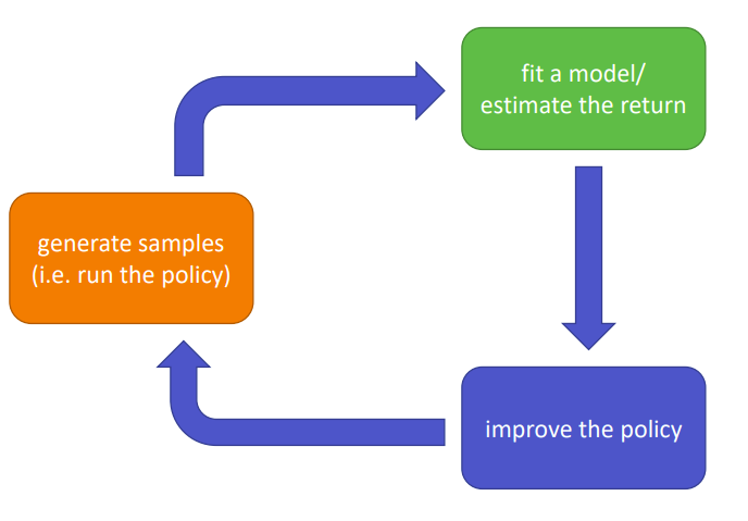
Figure 1: The anatomy of a RL algorithm
Given the objective of Eq. \ref{eq:finite_hor} or \ref{eq:inf_hor}, or some other variants such as discounted total reward, we can exploit different algorithms to optimize a policy:
- Policy Gradients: directly differentiate the objective function
- Value Based: estimate the value function or the $Q$ function of the optimal policy
- Actor-Critic: estimate the value or $Q$ function of the current policy, and use it to improve the policy
- Model Based: estimate the transition model of the environment and use it for planning, improving the policy, and more.
An important distinction to make is the one between on-policy and off-policy algorithms:
- Off-Policy: able to improve the policy using samples collected from different policies. These algorithms are more sample efficient because they need less samples from the environment.
- On-Policy: need to generate new samples every time the policy is changed, therefore require more samples.
It is important to note that better sample efficiency does not imply a better model. In some cases, generating new samples may be way faster than updating the policy (for example, when using big neural networks). Different algorithms make different assumptions on the state and action spaces as well as the nature of the task (episodic vs continuous). Moreover, convergence is not always guaranteed in many cases! One should always chose the algorithm by taking all this and much more factors into account.