- Actor: The policy $\pi$
- Critic: The value function $V^\pi$
Reducing Policy Gradient Variance
The REINFORCE algorithm seen in the previous lecture optimizes:
\begin{equation} \label{eq:basic_objective} \nabla_{\theta} J(\theta) \simeq \frac{1}{N} \sum_i^N \left( \sum_t \nabla_{\theta} \log \pi_{\theta} (a_{i, t} \mid s_{i, t}) \left( \sum_{t^{\prime}} r(s_{i, t^{\prime}}, a_{i, t^{\prime}}) \right) \right) \end{equation}
Nevertheless, it presents high variance and causality problems. We saw that using the estimate of the expected reward of the current state-action pair: $\hat Q^\pi (s_t^i, a_t^i)$ (i.e: reward-to-go) already reduced variance as it averages all possible trajectories values.
\begin{equation} \nabla_{\theta} J(\theta) \simeq \frac{1}{N} \sum_i^N \sum_t \nabla_{\theta} \log \pi_{\theta} (a_{i, t} \mid s_{i, t}) \hat Q^\pi (s_t^i, a_t^i) \end{equation}
We also saw the power of baselines to reduce variance: In particular, we can use the state-dependent baseline: $V(s_{i, t})$: critic-based estimator. With this, we indicate how much better the action $a_{i, t}$ is, with respect to the average action in state $s_{i, t}$, we refer to it as the advantage function:
\begin{equation} A^\pi (s_t, a_t) := Q^\pi (s_t, a_t) - V^\pi (s_t) \end{equation}
We cannot add an action-dependent bias like $Q^\pi (s_t, a_t)$ unless we add some other term to zero the expectation. More on this paper
Thus, where the better the estimate of $\hat A$ is, the lower the variance:
\begin{equation} \nabla_{\theta} J(\theta) \simeq \frac{1}{N} \sum_i^N \sum_t \nabla_{\theta} \log \pi_{\theta} (a_{i, t} \mid s_{i, t}) \hat A^\pi (s_t^i, a_t^i) \end{equation}
So, what should we fit, $Q^\pi$, $V^\pi$ or $A^\pi$?
PROS of $Q^\pi$:
- If you have $Q^\pi$, you can derive $V^\pi$ or $A^\pi$.
- $A^\pi$ is very dependent on your policy, $Q^\pi$ is more stable.
PROS of $V^\pi$:
- $Q^\pi$ and $A^\pi$ are bigger, depend both on states and actions, $V^\pi$ only on states.
- We can roughly approximate both $Q^\pi$ and $A^\pi$ with $V^\pi$:
- $Q^\pi (s_t, a_t) = r(s_t, a_t) + E_{s_{t+1} \sim p(s_{t+1} \mid s_t, a_t)} [V^{\pi} (s_{t+1})] \simeq r(s_t, a_t) + V^{\pi} (s_{t+1})$
- $A^\pi (s_t, a_t) \simeq r(s_t, a_t) + V^{\pi} (s_{t+1}) - V^{\pi} (s_t)$
If we don’t want to fit something that takes both states and actions we can just fit $V^{\pi}$ at the cost of using a single-sample estimate for $s_{t+1}$. We will do this for now, to fit $Q^\pi$ look into Q-learning methods.
Policy Evaluation
Fitting a value function $V^\pi$ for a given policy $\pi$. To do so we generate some training dataset: ${ (s_{i, t}, y_{i, t})} $. And use it to train an ANN which models $V^{\pi}$ in a supervised learning fashion.
Monte Carlo (MC) Policy Evaluation
Use single-sample estimate of return of a particular state:
\begin{equation} y_{i, t} = \hat V^{\pi} (s_t) \simeq \sum_{t^{\prime}=t}^T r(s_{t^{\prime}}, a_{t^{\prime}}) \end{equation}
If we approximate $V^{\pi}$ like this, isn’t that the same as what we were doing in Eq. \ref{eq:basic_objective} ? Not if we use a value function approximator able to generalize which doesn’t overfit (e.g. ANNs). It will average out similar states and generalize to unseen ones.
Bootstrapped Estimate Evaluation
Use previous value function approximation when updating current value function:
\begin{equation} y_{i, t} = \hat V^{\pi} (s_t) \simeq r(a_{i, t}, s_{i, t}) + \hat V_{\phi}^{\pi} (s_{i, t+1}) \end{equation}
Monte Carlo vs Bootstrapped Estimate
- Monte Carlo has a lower bias: It estimates $V^\pi$ from actual runs, while Bootstrapped Estimate uses past approximations of itself. Moreover, if the model approximating $\hat V^\pi$ has a bias its estimation will be biased as well.
- Bootstrapped Estimate has a lower variance: It averages rewards from multiple runs. Better for very stochastic policies or environments with a lot of noise.
Infinite Horizon Problems
If we keep adding rewards, $\hat V^{\pi} (s_t)$ will diverge to infinity (even worse for infinite-horizon problems). We can add a temporal discount factor \(\gamma \in [0, 1]\), usually around $\gamma \simeq 0.99$ which penalizes future rewards: “Better to get rewards sooner than later”.
Monte Carlo Estimate would then look like:
\begin{equation} y_{i, t} = \hat V^{\pi} (s_t) \simeq \sum_{t^{\prime}=t}^T \gamma^{t^{\prime} - t} r(s_{t^{\prime}}, a_{t^{\prime}}) \end{equation}
And bootstrapped estimate like:
\begin{equation} y_{i, t} \simeq r(a_{i, t}, s_{i, t}) + \gamma \hat V_{\phi}^{\pi} (s_{i, t+1}) \end{equation}
Actor-Critic (AC) Algorithm
With this, we can define an offline and an online learning method based on the REINFORCE algorithm but using an estimate of $V^\pi$ to evaluate $A^\pi$:
Batch actor-critic
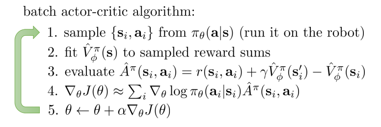
Figure 1: Batch actor-critic algorithm
Online actor-critic
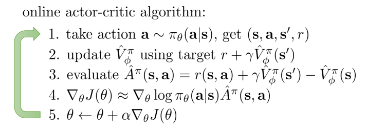
Figure 2: Online actor-critic algorithm
Notice that we need 2 ANNs, one for $\pi_\theta$ and one for $\hat V^\pi$.
We could make them share the first feature-extracting layers and have a single network with “2 heads”:
- Pros:
- Faster learning.
- Cons:
- Harder to implement.
- The combination of 2 learning gradients on a shared network can become unstable (how do you decide each learning rate? variance of policy gradient is much larger than the one in value gradients).
Online AC problem: We train using a minibatch size of 1 $\Rightarrow$ Not even Supervised Learning works if training with 1-sample batches!! (Too noisy) If we want a bigger batch size we need parallel sampling workers. We can use synchronized (easier to implement) or a asynchronous algorithm.
Eligibility traces and n-step returns
So far we know:
- Short-term samples have low variance (a sample of you doing something tomorrow is more accurate than one of in 30 years) $\Rightarrow$ MC excels short-term.
- Bias in long-term predictions is not as big of a problem compared to variance $\Rightarrow$ Bootstrapping excels long-term.
IDEA: Can we combine MC and Bootstrap to balance the bias-variance trade-off? Introducing n-step return estimator:
\begin{equation} A_n^{\pi} (s_t, a_t) = \sum_{t^{\prime} = t}^{t + n} \gamma^{t^{\prime} - t} r(s_{t^{\prime}}, a_{t^{\prime}}) - \hat V_{\theta}^{\pi} (s_t) + \gamma^n \hat V_{\theta}^{\pi} (s_{t+n}) \end{equation}
With n you can balance the bias-variance trade-off presented, but how do you choose n? You can average out all possible n values. Introducing Generalized Advantage Estimator (GAE):
\begin{equation} \hat A_{GAE}^{\pi} (s_t, a_t)= \sum_{n=1}^\infty w_n A_n^{\pi} (s_t, a_t) \end{equation}
The weights can also behave as a Geometric sequence (similar to discount factor $\gamma$): $w_n \propto \lambda^{n-1}$. After some algebra:
\begin{equation} \label{eq:gae} \hat A_{GAE}^{\pi} (s_t, a_t)= \sum_{t^{\prime} = t}^\infty (\gamma \lambda)^{t^{\prime} - t} \delta_{t^\prime} \end{equation}
Where:
\begin{equation} \delta_{t^\prime} = r(s_{t^{\prime}}, a_{t^{\prime}}) - \hat V_{\theta}^{\pi} (s_t) + \gamma^n \hat V_{\theta}^{\pi} (s_{t+1}) \end{equation}
$\gamma$ and $\lambda$ get multiplied together in Eq. \ref{eq:gae} $\Rightarrow$ they have similar effects $\Rightarrow$ they both balance the bias-variance trade-off $\Rightarrow$ discount factor is also a form of variance reduction.