In this lecture we take a deeper dive into why Policy Gradient algorithms work, and we extract some useful knowledge that will help us to derive advanced Policy Gradient algorithms such as Natural Policy Gradient, Trust Region Policy Optimization, or Proximal Policy Optimization.
Policy Gradient as Policy Iteration
Recalling the Policy Gradient in the Actor-Critic configuration \begin{equation} \nabla_{\theta}J(\theta) \approx \frac{1}{N} \sum_{i=1}^N \sum_{t=1}^T \nabla_{\theta}\log \pi_{\theta}(a_{i, t} \vert s_{i, t}) A^{\pi}_{i, t} \end{equation}
And can be seen as repeating the steps:
- Estimate \(A^{\pi}_{i, t}\) for current policy \(\pi\)
- Use \(A^{\pi}(s_t, a_t)\) to get improved policy \(\pi'\)
These steps are the same we do in Policy Iteration! We then want to understand under which conditions Policy Gradient is a Policy Iteration. In order to do this, we analyze the policy improvement of Policy Gradient.
The Policy Gradient objective is
\[J(\theta) = E_{\tau \sim p_{\theta}(\tau)}\left[ \sum_{t}\gamma^t r(s_t, a_t) \right]\]It can be shown (S. Levine’s Advanced Policy Gradients lecture, slide 6) that the policy improvement between the new policy parameters \(\theta'\) and the old \(\theta\) can be written as \begin{equation} \label{eq:improvement} J(\theta’) - J(\theta) = E_{\tau \sim p_{\theta’}(\tau)} \left[ \sum_t \gamma^t A^{\pi_{\theta}}(s_t, a_t) \right] \end{equation} That is the expected total advantage with respect to the parameters \(\theta\) under the distribution induced by the new parameters \(\theta'\). This is very important, because this improvement objective is the same of Policy Iteration. If we can show that the gradient of this improvement is the same gradient of Policy Gradient, then we can show that Policy Gradient moves in the direction of improving the same thing as Policy Iteration.
We therefore want to take the gradient of the improvement Eq. \ref{eq:improvement} in order to maximize it. However, the improvement is an expectation under the new parameters \(\theta'\), and we cannot compute it from the samples we have, that were obtained under the old parameters \(\theta\). To take the gradient of Eq. \ref{eq:improvement}, we need to write it as an expectation under the current parameters \(\theta\). With the usual properties of the expected value we expand:
\begin{equation} E_{\tau \sim p_{\theta’}(\tau)} \left[ \sum_t \gamma^t A^{\pi_{\theta}}(s_t, a_t) \right] = \sum_t E_{s_{t} \sim p_{\theta’}(s_{t})} \left[ E_{a_{t} \sim \pi_{\theta’}(a_{t})} \left[ \gamma^t A^{\pi_{\theta}}(s_t, a_t) \right]\right] \end{equation} We can now apply Importance Sampling to write the inner expectation over \(\pi_{\theta'}(a_t)\) as an expectation over \(\pi_{\theta}(a_t)\): \begin{equation} \label{eq:is} E_{\tau \sim p_{\theta’}(\tau)} \left[ \sum_t \gamma^t A^{\pi_{\theta}}(s_t, a_t) \right] = \sum_t E_{s_{t} \sim p_{\theta’}(s_{t})} \left[ E_{a_{t} \sim \pi_{\theta}(a_{t})} \left[ \frac{\pi_{\theta^{\prime}}(a_t)}{\pi_{\theta}(a_t)} \gamma^t A^{\pi_{\theta}}(s_t, a_t) \right]\right] \end{equation}
A careful reader would notice that there still is a problem: we still have the expectation over \(p_{\theta'}\). If the total variation divergence -sum of the absolute difference of each component- of \(\pi\) and \(\pi'\) is bounded by \(\epsilon\),
\[\vert \pi_{\theta'}(a_t \vert s_t) - \pi_{\theta}(a_t \vert s_t) \vert \le \epsilon\]then, the divergence of the stationary distributions \(p_{\theta'}\) and \(p_{\theta}\) is bounded:
\[\vert p_{\theta'}(s_t) - p_{\theta}(s_t) \vert \le 2\epsilon t\]Then, the objective difference of Eq. \ref{eq:improvement} is bounded
\[J(\theta') - J(\theta) \le \sum_{t} 2\epsilon t C\]where \(r_{max}\) is the maximum single reward obtainable, and \(C \in O(\frac{r_{max}}{1 - \gamma})\). If you are interested in the details of this derivation, check the Trust Region Policy Optimization paper. Therefore, we can substitute \(p_{\theta'}\) with \(p_{\theta}\) in the leftmost expectation of Eq. \ref{eq:is} and optimize the new objective \(\overline{A}(\theta')\) with respect to \(\theta'\):
\begin{equation} \label{eq:opt_objective} \overline{A}(\theta’) = \sum_t E_{s_t \sim p_{\theta}(s_t)}\left[ E_{a_t \sim \pi_{\theta}(a_t \vert s_t)}\left[ \frac{\pi_{\theta’}(a_t \vert s_t)}{\pi_{\theta}(a_t \vert s_t)} \gamma^t A^{\pi_{\theta}}(s_t, a_t) \right] \right] \end{equation}
\begin{equation} \label{eq:opt_A} \theta’ \leftarrow \arg\max_{\theta’} \overline{A}(\theta’) \end{equation}
A better measure of divergence
Unfortunately, it is not easy to compute the total variation divergence between two distributions, and we cannot therefore use it in practice. Therefore, in many implementations as well as theoretical papers, the KL Divergence is used. In fact, for two distributions \(\pi_{\theta'}(a_t \vert s_t)\) and \(\pi_{\theta}(a_t \vert s_t)\), we have that their total variation divergence is bounded by the square root of their KL divergence (written as \(D_{KL}\)).
\begin{equation} \vert \pi_{\theta’}(a_t \vert s_t) - \pi_{\theta}(a_t \vert s_t) \vert \le \sqrt{\frac{1}{2} D_{KL}\left(\pi_{\theta’}(a_t \vert s_t) \vert\vert \pi_{\theta}(a_t \vert s_t)\right)} \end{equation}
We can therefore use the KL Divergence instead of the total variation divergence to measure how “close” two policies are. In turn, the KL Divergence is easier to compute for many classes of distributions.
Enforcing the KL constraint
All the considerations above led us to a key insight: when optimizing Eq. \ref{eq:opt_A}, we must ensure that the optimization step does not drive the new policy \(\pi'\) too far from the previous \(\pi\). We therefore need to constrain the optimization such that
\begin{equation} \label{eq:kl_constraint} D_{KL}\left(\pi_{\theta’(a_t \vert s_t)} \vert \vert \pi_{\theta}(a_t \vert s_t)\right) \le \epsilon \end{equation}
Dual Gradient Descent
We can subtract the KL Divergence to the maximization objective of Eq. \ref{eq:opt_objective} \begin{equation} \label{eq:dual_opt} \mathcal{L}(\theta’, \lambda) = \overline{A}(\theta’) - \lambda \left(D_{KL}\left(\pi_{\theta’} (a_t \vert s_t) \vert\vert \pi_{\theta}(a_t \vert s_t)\right) - \epsilon\right) \end{equation}
and perform a dual gradient descent by repeating the following steps:
- Maximize \(\mathcal{L}(\theta', \lambda)\) with respect to \(\theta'\) (usually not until convergence, but only a few maximization steps)
- Update \(\lambda \leftarrow \lambda + \alpha \left( D_{KL}\left(\pi_{\theta'}(a_t \vert s_t) \vert\vert \pi_{\theta}(a_t \vert s_t)\right) - \epsilon \right)\)
Natural Gradients
One way to optimize a function within a certain range is, provided that the range is small enough, to take a first order Taylor expansion and optimize it instead. If we take a linear expansion of our objective and we evaluate it at \(\theta\), we obtain the usual Policy Gradient:
\begin{equation} \nabla_{\theta}\overline{A}(\theta) = \sum_t E_{s_t \sim p_{\theta}(s_t)}\left[ E_{a_t \sim p_{\theta}(a_t \vert s_t)} \left[ \gamma^t \nabla_{\theta}\log\pi_{\theta}(a_t \vert s_t) A^{\pi_{\theta}}(s_t, a_t) \right]\right] \end{equation} since the importance sampling ratio in \(\theta\) becomes 1. See Lecture 5: Policy Gradients for the gradient derivation.
Taking a Policy Gradient step means that we are taking a step in a circular radius around \(\theta\), which is equivalent of maximizing \(\overline{A}\) subject to \begin{equation} \label{eq:circle_constr} \vert\vert \theta’ - \theta \vert\vert^2 \le \epsilon \end{equation} However, our constraint is that of Eq. \ref{eq:kl_constraint}. We therefore take a second order approximation of the KL Divergence
\begin{equation} D_{KL}(\pi_{\theta’} \vert\vert \pi_{\theta}) \approx \frac{1}{2} (\theta’ - \theta) \pmb{F} (\theta’ - \theta) \end{equation} where \(\pmb{F}\) is the Fischer Information Matrix. This makes our optimization region becoming an ellipse inside which the KL constraint is respected.
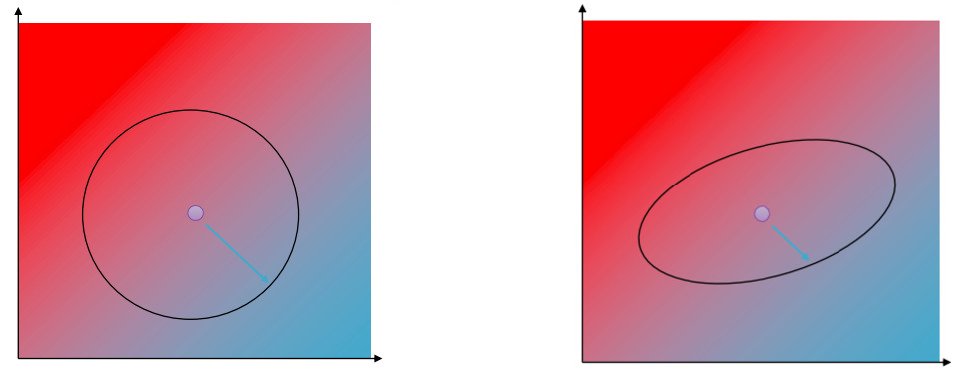
The figure above shows the optimization regions given, respectively, by the “naive” constraint of Eq. \ref{eq:circle_constr} implied by the and the usual Policy Gradient algorithm, and that given by the \(D_{KL}\) constraint of Eq. \ref{eq:kl_constraint}.
We transform our objective by \(\pmb{F}\) inverse, such that the optimiation region becomes again a circle and we can take a gradient step on this transformation. We call this the Natural Gradient:
\begin{equation} \theta’ = \theta + \alpha \pmb{F}^{-1} \nabla_{\theta}J(\theta) \end{equation} The learning rate \(\alpha\) must be chosen carefully. More on Natural Gradients in J. Peters, S. Schaal, Reinforcement learning of motor skills with policy gradients
The use of a natural gradient however does not come without its issues. The Fischer Information Matrix is defined as \begin{equation} \pmb{F} = E_{\pi_{\theta}}\left[ \nabla_{\theta}\log\pi_{\theta}(\pmb{a}\vert\pmb{s}) \nabla_{\theta}\log\pi_{\theta}(\pmb{a}\vert\pmb{s})^T \right] \end{equation} which is the outer product of the gradient logs. Therefore, if \(\theta\) has a million parameters, \(\pmb{F}\) will be a million by a million matrix, and computing its inverse would become infeasible. Moreover, since it is an expectation, we also need to compute it from samples, which again increases the computational cost.
Trust Region Policy Optimization
While in the paragraph above we chose the learning rate ourselves, we may want to instead choose \(\epsilon\) and enforce each gradient step to be ecactly \(\epsilon\) in \(D_{KL}\) variation. We therefore use a learning rate \(\alpha\) according to \begin{equation} \alpha = \sqrt{\frac{2\epsilon}{\nabla_{\theta}J(\theta)^T\pmb{F}\nabla_{\theta}J(\theta)}} \end{equation} Schulman et al., Trust Region Policy Optimization introduced the homonymous algorithm, and, most importantly, provides a efficient way of computing the matrix \(\pmb{F}\).
Proximal Policy Optimization
Schulman et al., Proximal Policy Optimization, proposes a way of enforcing the \(D_{KL}\) constraint without the need of computing the Fischer Information Matrix or its approximation. This can obtained in two ways:
Clipping the surrogate objective
Let \(r(\theta)\) be the Importance Sampling ratio of the Eq. \ref{eq:opt_objective} objective. Here, we maximize instead a clipped objective \begin{equation} L^{CLIP} = E_t \left[ \min\left( r_r(\theta)A_t, clip(r_t(\theta), 1-\epsilon, 1+\epsilon)A_t \right) \right] \end{equation}
The following figure shows a single term in \(L^{CLIP}\) for positive and negative advantage.
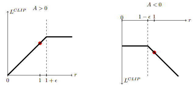
However, recent papers such as Engstrom et al., Implementation Matters in Deep Policy Gradients show how this clipping mechanism does not prevent the gradient steps to violate the KL constraint. Furthermore, they claim that the effectiveness that made PPO famous comes from its code-level optimizations, and TRPO above may actually be better if these are implemented.
Adaptive KL Penalty Coefficient
Another approach described by the PPO paper is similar to the dual gradient descent we described above. It consists in repeating the following steps in each policy update:
- Using several epochs of minibatch SGD, optimize the KL-penalized objective
- Compute \(d = E_t \left[ D_{KL}(\pi_{\theta'}(. \vert s_t)\vert\vert
\pi_{\theta}(. \vert s_t)) \right]\)
- If \(d \lt d_{targ}/1.5\) then \(\beta \leftarrow \beta/2\)
- If \(d \gt 1.5 d_{targ}\) then \(\beta \leftarrow 2\beta\)
Where \(d_{targ}\) is the desired KL Divergence target value.