Autoregressive models (AR)
Given a dataset \(\mathcal{D} = \{x^1, ... x^K \}\) of K n-dimensional datapoints \(x\) (\(x\) could be a flattened image for instance) we can apply the chain rule of probability to each dimension of the datapoint (we take the density estimation perspective):
\begin{equation} p(x) = \prod_i^n p(x_i \mid x_{< i}) \end{equation}
Autoregressive models fix an ordering of the variables and model each conditional probability \(p(x_i \mid x_{< i})\). This model is composed by a parametrized function with a fixed number of params. In practice fitting each of the distributions is computationally infeasible (too many parameters for high-dimensional inputs).
This decomposition converts the joint modelling problem \(p(x_1, ..., x_n)\) into a sequence modeling one.
A Bayesian network which does not do any assumption on the conditional independence of the variables is set to obey the autoregressive property.
Simplification methods:
-
Independence assumption: Instead of each variable dependent on all the previous, you could define a probabilistic graphical model and define some dependencies: \(P(x) \simeq \prod_i^n p \left(x_i \mid \{ x_j \}_{j \in parents_i} \right)\). For instance, one could do Markov assumptions: \(P(x) \simeq \prod_i^n p \left(x_i \mid x_{i-1} \right)\). More on this paper and this other paper.
-
Parameter reduction: To ease the training one can under-parametrize the model and apply VI to find the closest distribution in the working sub-space. For instance you could design the conditional approximators parameters to grow linearly in input size like: \(P(x) \simeq \prod_i^n p \left(x_i \mid x_{< i}, \theta_i \right)\) where \(\theta_i \in \mathcal{R}^i\). More of this here.
-
Increase representation power: I.e. parametrize \(p(x_i \mid x_{< i})\) with an ANN. Parameters can either remain constant or increase with \(i\) (see figure 2). In addition you can make these networks share parameters to ease the learning.
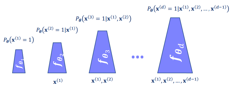
Figure 2: Growing ANN modelling of the conditional distributions. (Image from KTH DD2412 course)
The order in which you traverse the data matters! While temporal and sequential data have natural orders, 2D data doesn’t. A solution is to train an ensemble with different orders (ENADE) and average its predictions.
Instead of having a static model for each input, we can use a RNN and encode the seen “context” information as hidden inputs. They work for sequences of arbitrary lengths and we can tune their modeling capacity. The only downsides are that they are slow to train (sequential) and might present vanishing/exploding gradient problems.
PixelRNN applies this idea to images. They present some tricks like multi-scale context to achieve better results than just traversing the pixels row-wise. It consists of first traversing sub-scaled versions of the image to finally fit the model on the whole image. If interested, check out our LMConv post. Some other interesting papers about this topic: PixelCNN WaveNet
Overall AR provide:
- Tractable likelihoods: exact and simple density estimation)
- Simple generation process, which is very good for data imputation (specially if available data is at the beginning of the input sequence)
But:
- There is no direct mechanism for learning features (no encoding).
- Slow: training, sample generation, and density estimation. Because of the sequential nature of the algorithm.