LMConv: Locally Masked Convolutions for Autoregressive Models
If not familiar with autoregressive generative models I suggest to first take a look at our Parametric Deep Generative Models post.
Idea
Remember: Given a dataset \(\mathcal{D} = \{x^1, ... x^K \}\) of K n-dimensional vectors, autoregressive generative models learn its underlying distribution \(p(x)\) by making use of the chain rule of probability:
\begin{equation} \label{eq:chain} p(x) = \prod_i^n p(x_i \mid x_{< i}) \end{equation}
Each of these conditional probabilities \(p(x_i \mid x_{< i})\) can be modelled by a single RNN. We can use this tractable \(p(x)\) for sample density estimation, sample new datapoints or missing data completion. In particular, this paper is interested in natural image completion.
Problem: Sequentially learning \(p(x_i \mid x_{< i})\) is order-dependent. While temporal and sequential data have natural orders, 2D data (such as images) doesn’t. Previous work (e.g. PixelRNN or PixelCNN) only trains on raster scan order (left to right, top to bottom). But this is only \(1\) of the \(n!\) possible image traversal ordering! This means inference can only be “reliably” done in this order. Therefore, it fails in image-completing tasks when it cannot observe the context (i.e. data is missing around first traversed pixels):
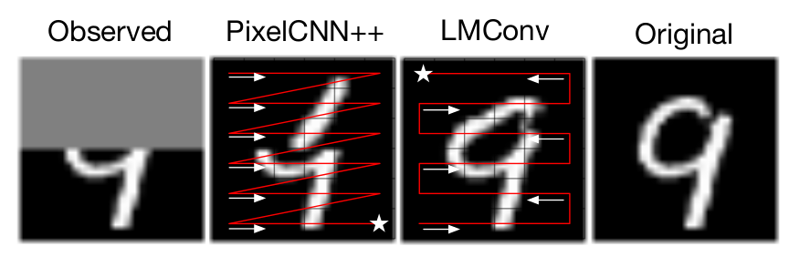
Figure 1: PixelCNN++ failing at image completion task because it cannot take advantage of the information in last rows of the image. LMConv can work in any order and uses all the available information to complete the image.
This work addresses this issue by adding 2 new ideas to PixelCNN: Train the model on different traversal order permutations, and use masking on the level of features.
Convolutional autoregressive networks transform a \(H \times W \times c\) image into a \(H \times W \times (c \cdot bins)\) log-probability tensor. Where \(bins\) is a discretization fo the light intensity of each channel. Row \(i\), column \(j\), depth \(k\%c\) indicate the log-probability of light intensity being in bin \(k\) for channel \(c\) in pixel \((i, j)\).
Pixel traversal permutation training
The idea is simple: train in arbitrary orders so that later the traversal can be customized to each task. For instance, in an image completion task one can obtain a richer context by first traversing the known pixels.
To do so, the authors define a set of traversal permutations \(\pi\) and assign a uniform distribution over them \(p_\pi\). They then apply MLE to:
\begin{equation} \mathcal{L} (\theta) = E_{x \sim p_{data}} E_{\pi \sim p_\pi} \log p_\theta (x_1, …, x_D ; \pi) \end{equation}
Where \(\log p_\theta (x_1, ..., x_D ; \pi)\) factorizes as depicted in eq. \ref{eq:chain} in following the order dictated by \(\pi\):
\begin{equation} \log p_\theta (x_1, …, x_D ; \pi) = \sum_i p_\theta (x_{\pi(i)} \mid x_{\pi(1)},…, x_{\pi(i-1)}) \end{equation}
Each of the conditionals are parametrized by the same RNN.
Local masking
Since the network is modelling \(p_\theta (x_{\pi(i)} \mid x_{\pi(1)},..., x_{\pi(i-1)})\) but we apply a convolution operation over the pixels, we need to make sure that when computing \(p_\theta (x_{\pi(i)} \mid x_{\pi(1)},..., x_{\pi(i-1)})\) we do not use information of any pixel other than \(x_{\pi(1)},..., x_{\pi(i-1)}\). Otherwise, if we make the probability depend on successors on the Bayesian network, the product of conditionals would be invalid due to cyclicity.
Previously this had been dealt in 2 different ways:
- NADE does \(D\) passes for each image. When evaluating \(p_\theta (x_{i} \mid x_{1},..., x_{i-1})\) they masks pixels \(x_{i+1},...,x_{D}\) to ensure no successor information is used.
- PixelCNN controls information flow by setting certain weights to the convolution filters to 0. This induces blind spots in the image generation which damage its performance.
Instead, this paper takes advantage of the implementation of the convolution operation to mask the corresponding values of the first-layer input. Essentially, convolutions are implemented as a general matrix multiplication (GEEM):
\begin{equation} Y = \mathcal{W} \cdot im2col (X, k_1, k_2) + b \end{equation}
Where: \(\mathcal{W}\) rows are each conv2D filter weights and \(b\) its biases. \(im2col (X, k_1, k_2)\) converts the input image \(X\) of shape \(H \times W \times c\) into a tensor of shape \((k_1 \cdot k_2 \cdot c) \times (H \cdot W)\). This tensor columns are the \((k_1 \times k_2 \times c)\) patches where the convolution filter is applied to.
The mask is applied before computing the convolution: \(\mathcal{M} \circ im2col (X, k_1, k_2)\). Its coefficients are dependent on the permutation \(\pi\) in which we are traversing the image at that iteration.
I oversimplified the algorithm for the seek of brevity, I recommend taking a look at the paper since the idea is quite smart. Be careful though, things get a bit convoluted (pun intended).
This allows for parallel computation of the conditionals.
Results
Density estimation
Tractable generative models are usually evaluated via the average negative log-likelihood (NLL) of test data:
-
This paper achieves marginally better NLL scores than PixelCNN++ on MNIST and CIFAR10. Furthermore they outperform Glow (read our post) in high-resolution imge dataset: CelebA-HQ. Nevertheless, they are still a bit behind against high-resolution specialized architectures such as SPN, which use self-attention.
-
They show training with 8 different orders achieves better results than a single one (even when evaluating test sample likelihood in a single order).
Novel orders generalization
-
Training on 8 S-curve orders and testing on a raster scan order results in a \(26\%\) NLL increase. (vs. \(26\%\) NLL increase if only trained with 1 S-curve)
-
Training on 7 s-curves and testing on a different s-curve results in a \(5\%\) NLL increase.
Image completion
- This work achieves better qualitative and NLL scores than PixelCNN++.
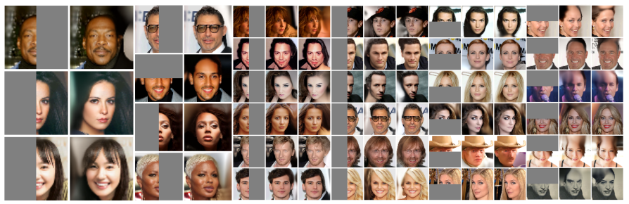
Figure 2: Missing pixels are generated along an s-curve which first traverses the observable regions.
Contribution
- Extension of PixelCNN to estimate more reliable likelihoods in arbitrary orders.
Weaknesses
-
Since it seems that they mostly care about image completion, I would like to see a comparison against a self-supervised network trained to specifically do so (different from other AR approaches, e.g. VAE).
-
I also wonder how transferable are the learned weights through different datasets. They only tested on 3 different datasets and re-trained each time the model.