Normalizing flow models
The main idea is to learn a deterministic bijective (invertible) mapping from easy distributions (easy to sample and easy to evaluate density, e.g. Gaussian) to the given data distribution (more complex).
First we need to understand the change of variables formula: Given \(Z\) and \(X\) random variables related by a bijective (invertable) mapping \(f : \mathbb{R}^n \rightarrow \mathbb{R}^n\) such that \(X = f(Z)\) and \(Z = f^{-1}(X)\) then:
\begin{equation} p_X(x) = p_Z \left( f^{-1} (x) \right) \left|\det \left( \frac{\partial f^{-1} (x)}{\partial x} \right)\right| \end{equation}
Were \(\frac{\partial f^{-1} (x)}{\partial x}\) is the \(n \times n\) Jacobian matrix of \(f^{-1}\). Notice that its determinant models the local change of volume of \(f^{-1}\) at the evaluated point.
“Normalizing” because the change of variables gives a normalized density after applying the transformations (achieved by multiplying with the Jacobian determinant). “Flow” because the invertible transformations can be composed with each other to create more complex invertible transformations: \(f = f_0 \circ ... \circ f_k\).
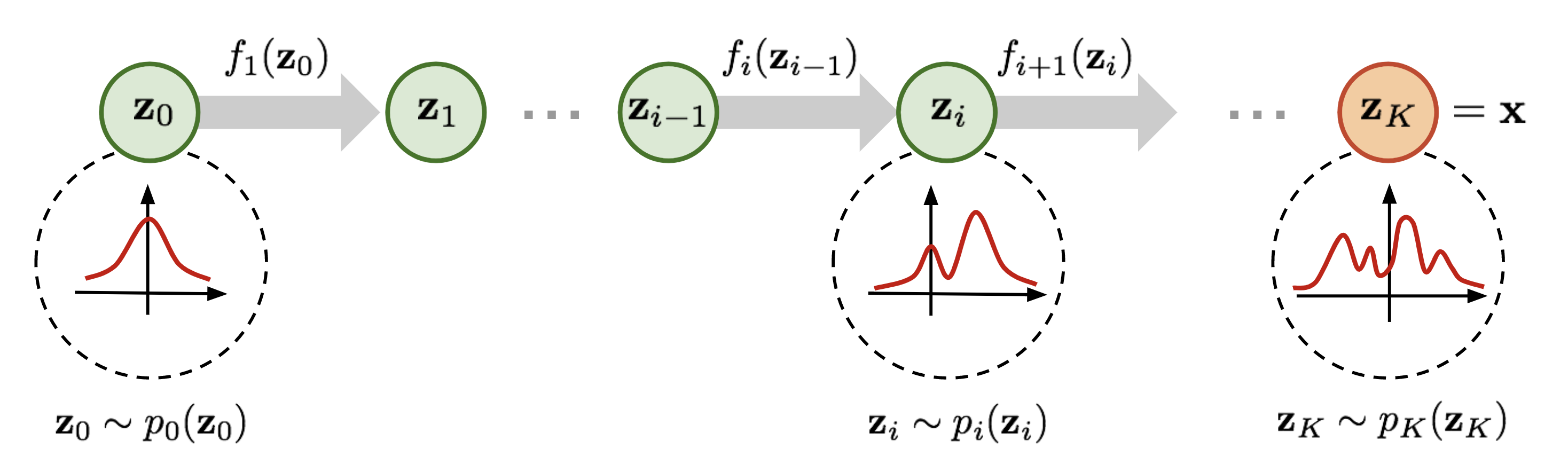
Figure 3: Normalizing flow steps example from 1D Gaussian to a more complex distribution. (Image from lilianweng.github.io)
As you might have guessed, normalizing flow models parametrize this \(f\) mapping function using an ANN \((f_\theta)\). This ANN, however, needs to verify some specific architectural structures:
- Needs to be deterministic
- I/O dimensions must be the same (\(f\) has to be bijective)
- Transformations must be invertible
- Computation of the determinant of the Jacobian must be efficient and differentiable.
Nevertheless they solve both previous approach problems:
- Present feature learning.
- Present a tractable marginal likelihood.
Most famous normalizing flow architectures (NICE, RealNVP, Glow) design layers whose Jacobian matrices are triangular or can be decomposed in triangular shape. These layers include variations of the affine coupling layer, activation normalization layer or invertible 1x1 conv. Check out our Glow paper post for further details on these layers.