Glow: Generative Flow with Invertible 1x1 Convolutions
If not familiar with flow-based generative models I suggest to first take a look at our Normalizing FLows post.
Idea
This paper presents a flow-based deep generative model extending from NICE, RealNVP algorithms. Its main novelty its the design of a distinct flow implementing a new invertible 1x1 conv layer.
The proposed flow is composed by a multi-scale architecture (same as in RealNVP where each step has 3 distinct flow-layers combined:
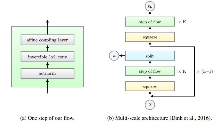
Figure 1: Each step of the proposed flow consists of three layers: an actnorm, the new invertible 1x1 conv and an affine coupling layer
Layers
Remember than in normalizing flows we look for bijective (invertible), deterministic, differentiable operations with an easy to compute Jacobian determinant.
Activation normalization (actnorm)
Applies a scale \(s_c\) and bias \(b_c\) parameter per channel \(c\) of the input. It is very similar to a batch normalization layer. The parameters are learnt (when maximizing flow likelihood) but they are initialized so that they set 0 mean and 1 std dev to the first data batch (data-dependent initialization).
Affine coupling layers
Given a D-dimensional input \(x\), this layer applies the following operations:
- Split \(x\) into 2 sub-vectors: \(x_{1:d}, x_{d+1:D}\)
- The first part \((x_{1:d})\) is left untouched.
- The second part undergoes an affine transformation (scale \(s\) and translation \(t\)). This scale and translations are a function dependent on the first part of the input vector: \(s(x_{1:d}), t(x_{1:d})\).
Overall:
\begin{equation} y_{1:d} = x_{1:d} \end{equation}
\begin{equation} y_{d+1:D} = x_{d+1:D} \circ \exp (s(x_{1:d})) + t(x_{1:d}) \end{equation}
The inverse is trivial and its Jacobian a lower triangular matrix (log-determinant is then the addition of the log-elements of the diagonal).
To ensure each dimension can affect each other dimension, we need to perform enough steps of some kind of permutations on the inputs. Previous work implemented a fixed simple permutation layer, this work generalizes this permutation by introducing the invertible 1x1 convolution.
Invertible 1x1 2D-convolution
This layer is a generalization of a permutation along the channels dimension. Given an input of shape \(h\times w \times c\). It applies a 1x1 convolution with \(c\) filters, meaning the output tensor shape is also going to be \(h\times w \times c\) (we need to keep the dimensions in normalizing flows).
Thus, each layer has a set of weights \(W\) with \(c \cdot c\) values. Its log-determinant can be computed as:
\begin{equation} \log \left| det \left( \frac{\partial conv2D(x; W)}{\partial x} \right) \right| = h\cdot w \cdot \log| (W) | \end{equation}
Its inverse operation can be computed by simply applying a convolution with \(W^{-1}\) weights.
Usually \(c=3\) so the \(det(W)\) and \(W^{-1}\) are cheap to compute.
Rather than a 1x1 2D-conv, I find it easier to imagine as: each channel of the output tensor is going to be a linear combination of the channels of the input tensor.
Layers summary
In summary this is each layer function, its inverse and its Jacobian log-determinant:
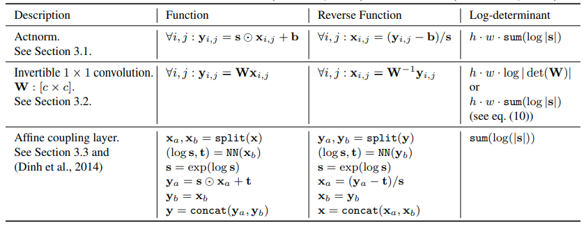
Figure 2: Layer summary
Results
Quantitative
The authors first show that:
-
Using the Invertible 1x1 2D-convolution achieves lower NLL scores when compared to fixed shuffles and reverse layers.
-
Affine coupling achieves lower NNL compared to additive coupling.
-
Glow achieves around 8.5% lower NNL compared to RealNVP averaged around common image datasets.
Qualitative
They test their algorithm on CelebA-HQ dataset (30000 celeb images of \(256^2\) px).
Synthesis and Interpolation
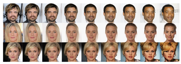
Figure 3: Smooth interpolation in latent space between two real images examples.
Semantic Manipulation
Each image has a binary label indicating the presence or absence of some attribute. For instance whether the celeb is smiling or not. Let \(z_{pos}\) be the average latent space position of samples presenting the attribute, and \(z_{neg}\) the average of the samples which do not present it. we can use the difference vector \(z_{pos} - z_{neg}\) as a direction on which to manipulate the samples to modify that particular attribute:
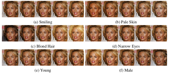
Figure 4: Attribute manipulation examples.
Temperature
When sampling they add a temperature parameter \(T\) and modify the distribution such that: \(p_{\theta, T} \propto \left( p_\theta (x)\right)^2\). They claim lower \(T\) values provide higher-quality samples:
Figure 5: Temperature parameter effect.
Contribution
-
Design of a new normalizing-flow layer: The invertible 1x1 convolution.
-
Improved quantitative SOTA results (in terms of log-likelihood of the modelled distribution \(P(X)\)).
Weaknesses
-
As this paper is more an evolution rather than a revolution there are no major weaknesses. Future lines of work could focus on the design of new normalizing flow layers and experiment on those.
-
They could further investigate the role of the temperature parameter \(T\).