ML Essentials
This post contains some key concepts using when dealing with ML models.
Basics
Machine Learning studies algorithms which improve their performance through data: The more data they process, the better they will perform.
- Paradigms of Machine Leaning:
- Supervised: Learns a mapping between a set of provided inputs and expected outputs: Used in regression and classification tasks.
- Unsupervised: Learn patters in unstructured data: clustering, dim-reduction, infer distributions…
- Reinforcement: Deals with decision-making problems.
To put it in simple terms:
- Supervised learning is predictive
- Unsupervised learning is descriptive
- Discriminative vs Generative:
- Discriminative models learn to map inputs to labels.
- Generative models learn the underlying distribution of the data. This allows us to perform density estimation, sampling, infer latent vars… Often used in unsupervised learning applications.
More on our Why generative models? post
- Bias-variance tradeoff:
- Bias is introduced by our choices on the model’s functional form. Wrong (or too-simple) assumptions often lead to under-fitting.
- Variance error is the opposite: it appears when the model is too susceptible to the data. For instance, over-parametrized models tend to over-fit to the training data and perform poorly on test data.
- Generalization: Ability of a model to perform well on untrained data.
- Bias error example: If you choose a linear model to capture non-linear relations, doesnt matter how much data you use to train, it will never fit it well.
- Variance error example: Decision trees are high-variance low-bias models, as they don’t do any assumption on the data structure. Usually its high variance is reduced through variance-reduction ensemble methods such as Bagging (further improved by Random Forests, where not only subsets of data are used but also subsets of features).
Optimizers
Optimizer is the algorithm which allows us to find the parameters which minimize an objective function. Very simple models might have a closed solution, which one should (obviously) use instead of these general techniques. Optimizers are often categorized by the order of the gradient available.
0-order
0-order optimizers are used when the gradients of the objective to optimize are not available (black box functions). These algorithms are often used in ML to optimize model meta-parameters, from which computing the gradient is not feasible or too expensive
- Random Search: Try multiple points and select the minimum value ever obtained.
- Grid Search: Evenly split the search space and evaluate the objective function at each point. A finer refinement can be done at the most promising area.
- Bayesian Optimization:
- Models the objective to optimize with a random function: for each point in the domain it encodes expected and uncertainty values. Usually Gaussian Processes are used (better calibrated than ANNs)
- First, a prior distribution is assumed for the random function, then, through iterative evaluations of the objective, the random function is approximated to the objective one.
- The acquisition function decides which point to evaluate at each iteration and varies depending on our goal: Expected Improvement, Lower Confidence Bound, Probability Improvement…
- Ideal for expensive-to-evaluate derivative-free functions (e.g. ANN meta-parameters)
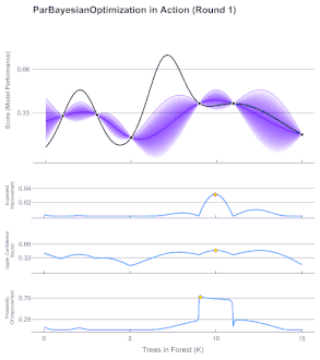
Bayesian Optimization Iteration
Another group of “fun” gradient-free optimizers are the meta-heuristics:
- Hill Climbing: Start at random point, greedily try to move towards a minimum by evaluating neighborhood positions.
- Genetic/Evolutionary: Start by evaluating a set of $n$ random solutions, choose the best among them and combine them (somehow) to create $n$ other solutions, repeat.
- Simulated Annealing: Move through the solution space allowing for miss-steps according to a decreasing “temperature” parameter.
- Ant colony: Have multiple agents trying solutions “leaving a trail” of their path proportional to their success to balance exploration and exploitation.
- There are many other meta-heuristic algorithms such as Particle Swarm, Tabu Search…
1st-order
They use the gradient of the objective (wrt the model’s weights) function in order to find the local minima. Most of the algorithms are based on gradient descent: Move in the direction of the steepest gradient. There are some variations to improve performance:
- Stochastic Gradient Descent: Make a gradient step after each input evaluation. Higher fluctuation (Higher variance).
- Mini-Batch Gradient Descent: Compute the gradient after evaluating a small subset of the training data (nicer balance).
- Momentum: Run an exponential moving average to smooth the computed gradient.
- ADAGRAD (ADAptative Gradient): Dynamically adjusts the learning rate.
- ADAM (ADAptative Model): Dynamically adjusts momentum.
Often, very deep or recurrent networks suffer from vanishing gradient problems:
- As the gradient gets back-propagated through the network, it is multiplied by the weight matrices at each step (derivative chain rule).
- If these weights are smaller than 1, the gradient “vanishes” and doesn’t have much impact on updating the network’s early layers’ weights.
Solutions:
- Use ReLU
While less frequent, if the weights of the network are bigger than 1, we can have an exploding gradient problem (completely analogous).
2nd-order
They use second order derivatives (Hessian). A common algorithm is to look for a $0$ of the objective’s derivative using the Netwon-Raphson method. As a reminder, if \(f\) is the derivative of our objective function, Newton-Raphson iteratively finds a $0$ as:
\begin{equation} x_{n+1} = x_n - \frac{f(x_n)}{f^\prime (x_n)} \end{equation}
2nd-order methods approximate quadratically the local neighborhood of the evaluated point while 1st-methods only approximate it linearly.
Pos/Cons:
- Local curvature information yields better performance (fewer steps)
- Doesn’t get stuck in critical points as much as 1st-order methods.
- Computationally expensive.
Since ANNs are already quite expensive to evaluate 2nd-order optimization methods are not used
Regularization
Techniques to improve model generality by imposing extra conditions in the training phase. These techniques reduce variance at the cost of higher bias.
L1 & L2
These regularization techniques are based on the idea of shrinkage: force the smaller (thus less-important) model parameters to zero to reduce variance. In regression tasks, this can be achieved by adding the norm of the weights to the loss function to optimize.
It is interesting to notice that shrinkage is implicit in Bayesian inference (dictated by the chosen prior).
Most famous methods are:
- Ridge regression: Uses the \(L_2\) norm. If working on a Bayesian framework (MAP), it is equivalent of choosing a Gaussian distribution for the weight’s prior. There is an essentially equivalent method to this called weight decay.
\begin{equation} \mathcal{L}^{\text{REG}} = \mathcal{L} + \lambda \Vert W \Vert_2^2 \end{equation}
- LASSO regression (Least Absolute Shrinkage and Selection Operator): Uses the \(L_1\) norm. If working on a Bayesian framework (MAP), it is equivalent of choosing a Laplace distribution for the weight’s prior.
\begin{equation} \mathcal{L}^{\text{REG}} = \mathcal{L} + \lambda \Vert W \Vert_1 \end{equation}
Interestingly, the L1 term is better at forcing some parameters to 0. Thus, LASSO regression can also be used for feature selection: detect which dimensions matter the most for the regression task we are working with.
Notice that this idea of penalizing high weights of the model by adding a term on the loss function can be also used in more complex models such as ANNs. Most ANN packages include the option to add regularization to a Dense layer.
$\lambda$ controls how strong the regularization applied is:
- High $\lambda \rightarrow$ High bias.
- Low $\lambda \rightarrow$ High variance.
Notice this is just a Lagrange multiplier parameter we use to optimize with the added constrain of forcing weights to be small.
Dropout
At each training iteration it randomly selects a subsets of the neurons and sets their output to $0$. This forces the network to learn multiple ways of mapping input and outputs, making it more robust.
Early stopping
This can be also thought as an ensemble technique since one might argue that we are training multiple models at once, one for each active set of neurons.
Split the data into three sets: training, evaluation and testing. Update model parameters based on training loss but stop training as soon as evaluation loss stops to decrease (there are multiple heuristics to detect this). Early stopping prevents the model to overfit to the training set.
Data Augmentation
To improve the network generality it is often a good idea to train with small randomly-perturbed inputs. In the case of images these perturbations could be:” random noise, translations, rotations, zoom, mirror…
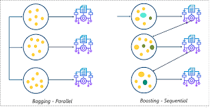
Ensemble Methods
Combine multiple weak learners to improve results. This can also be seen as a type of regularization, as averaging over multiple models boosts generality.
-
Mode: Simple voting mechanism. Take what the majority of learners say
-
Average / Weighted Average: Assign a weight to each learner and compute the mean prediction.
-
BAGGING (Bootstrap AGGregatING) : Multiple models of the same type are trained with a random subset of the data sampled with replacement (bootstrapping). This technique is specially effective to reduce variance.
-
BOOSTING (aka Arcing (Adaptive Reweighting and Combining)): Trains models sequentially based on previous model performance instead of in parallel such as Bagging.
-
ADABOOST: Each datapoint is given an “importance weight” which is adjusted during the sequential training of multiple models: Missclassified datapoints are assigned a higher weight to make subsequent models consider them more. In addition, a “reliability weight” is assigned to each model and weighted average is used for the final guess. Although it also lowers the variance, it is mainly used to lower the bias of the models.
-
Gradient Boosting (GB): Instead of changing the weight of each missclassified input-label pair, GB sequentially fits each model to match the error given by the previous model. So if real labels are $y_i$ and the first model is trained on $x_i$ and outputs $h_i$, the second model will attempt to map $x_i$ to $y_i - h_i$. The final prediction is then given by the addition of the output of all models.
-
BAGGING vs ADABOOST
Error Measures
In this section we will take a look at the most common model criteria
Loss functions
Regression
- MAE (Mean Absolute Error): \(\mathcal{L} = \frac{1}{n} \sum_i \vert y_i - \hat y_i \vert\)
- Harder for the optimizer than MSE (non-differentiable)
- Goes more easy on outliers than MSE since it does not square them
- MSE (Mean Squared Error): \(\mathcal{L} = \frac{1}{n} \sum_i ( y_i - \hat y_i )^2\)
- Used in linear regression
- MSLE (Mean Squared Logarithmic Error): \(\mathcal{L} = \frac{1}{n} \sum_i ( \log (y_i + 1) - \log( \hat y_i + 1) )^2\)
- If you do not want to penalize as much bigger differences in larger numbers
Classification
- Cross-Entropy: \(\mathcal{L} = \frac{1}{n} \sum_i \sum_k y_i^k \log (\hat y_i^k)\)
- Measures distance between two distributions (real and guessed).
- Special case of KL divergence where data’s entropy is assumed to be 0.
- KL Divergence: \(\mathcal{L} = \frac{1}{n} \sum_i \sum_k y_i^k \log (\hat y_i^k) - \frac{1}{n} \sum_i \sum_k y_i^k \log (y_i^k)\)
- Measures “distance” between two distributions
- NLL (Negative Log-Likelihood): \(\mathcal{L} = \frac{1}{n} \sum_i \log (\hat y_i^{\text{true}})\)
- Same as cross-entropy applied to a 1-hot encoding of the classes
- Cosine similarity: \(\mathcal{L} = \frac{y}{\Vert y \Vert^2} \frac{\hat y}{\Vert \hat y \Vert^2}\)
- Measures the angle between two vectors (ignoring their magnitudes)
- Hinge Loss: \(\mathcal{L} = \frac{1}{n} \sum_i \max ( 0, m - y_i \hat y_i )\)
- Where $m$ is a margin value
- Is the loss used to optimize SVM
Cross-validation
Cross-validation splits the data into n equal chunks and trains n different times the algorithm, each time leaving a chunk for testing. Finally, we can get an idea on how good the model performs by averaging the loss functions obtained in every test.
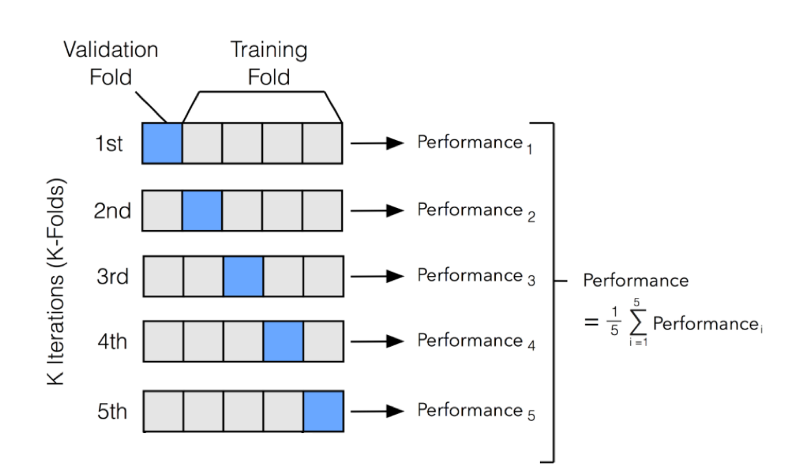
Cross validation approach to model testing
If we have as many chunks as datapoints, we call it leave-one-out cross-validation.
It is useful to compare the performance of different models being economic on the available data. It is also used to optimize hyper-parameters.
Binary Confusion Matrix
For binary classification tasks it is very useful to construct the binary confusion matrix and compare different model performances with the following metrics:
- Type I Error: False Positive (Model guessed + but was -).
- Type II Error: False Negative (Model guessed - but was +).
- Accuracy: \(\frac{\text{TP} + \text{TN}}{\text{TOTAL}}\). Overall, what proportion did the model correctly guess.
- Precision: \(\frac{\text{TP}}{\text{TP} + \text{I}}\). From the ones, you said were +, what proportion did you correctly guess.
- Recall: \(\frac{\text{TP}}{\text{TP} + \text{II}}\). From the ones that were +, how many did you correctly guess. (aka true positive rate (TPR))
- Specificity: \(\frac{\text{TN}}{\text{TN} + \text{I}}\). From the ones that were -, how many did you correctly guess.
Receiving Operating Characteristic ROC
Compares model Recall vs FPR (1 - Specificity) obtained with the studied model when varying a parameter.
- AUC Measures how good is the model at distinguishing the classes. Higher AUG means higher RECALL and higher SPECIFICITY: Which means it is better at predicting positives as positives and negatives as negatives.