CampusAI

Notation: I will refer to datapoints as $x$ (usually high-dimensional), labels as $y$ and latent variables as $z$. Notice the similarity between $y$ and $z$, the only difference being $y$ are explicitly provided and $z$ are intrinsic to the data (hidden).

Basics

Generative models fall in the realm of unsupervised learning: A branch of machine learning which learns patterns from unlabeled data. Most common unsupervised learning algorithms concern: clustering, dimensionality reduction, or latent variable models.

Before venturing in more complex details of generative models, lets take a moment to refresh Bayes formula:

\begin{equation} P(y | x) = \frac{P(x | y) P(y)}{P(x)} \end{equation}

Naming goes: Posterior: $P(y \mid x)$. Likelihood: $P(x \mid y)$. Prior: $P(y)$. Evidence: $P(x)$.

Discriminative vs Generative models

Discriminative models task is to predict a label $y$ for any given datapoint $x$. I.e. learn the conditional probability distribution $P(y \mid x)$ (posterior) by mapping inputs to provided labels. Most Supervised learning models are discriminative.
Generative models attempt to learn an approximate probabilistic distribution of $P(x)$, $P(x \mid z)$, or $P(z \mid x)$. Usually some functional form of $P(z)$ and $P(X \mid z)$ is assumed, then their parameters are estimated using data. If interested in the posterior one can use Bayes to compute it. Most Unsupervised learning models are generative.

Discriminative models usually outperform generative models in classification tasks:

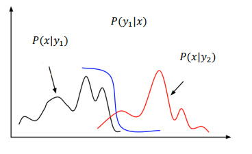
Figure 1: Learning a decision boundary $P(y \mid x)$ is easier than learning the full x distribution of each class $P(x \mid y)$ (Image from KTH DD2412 course)

Nevertheless the rich interpretation generative models do of our data can be very useful. The next section presents some of their use-cases.

Generative models use-cases

So, imagine we have a dataset $\mathcal{D}$ of dog images and an algorithm capable of modelling its underlying distribution: $P(X)$. We could:

Sample new datapoints from $P(X)$ distribution. For instance, we could obtain new dog images beyond the observed ones by sampling from our modelled “dog image distribution”.
Evaluate the probability of a sample $x$ by $P(x)$ (density estimation). We could use this to check how likely it is that a given image comes from the “dog image distribution” we used for training. Can be useful in uncertainty estimation to detect out-of-distribution (OOD) samples.
Infer latent variables $z$. In the dog example we could understand the underlying common structure of dog images. These latent variables could be dog position, fur color, ears type…

Quantitative evaluation of generative models is non-trivial and is still being researched on. A common evaluation metric of $P_\theta(x)$ is to assess the negative log-likelihood (NLL) of a “test” set. Images from a dataset should have very high likelihood (they are samples of the distribution).

Not all type of generative models are able to perform all of the above use-cases. There exist many different approaches (types) with their strengths and weaknesses.

Generative model types

Likelihood-based methods

They try to optimize the likelihood of the observed data for each data-point:

\begin{equation} \mathcal{L} (x_i) = - \log p_\theta (x_i) \end{equation}

Where:

\begin{equation} p_\theta (x_i) = \int_z p_\theta (x_i \mid z) p(z) dz \end{equation}

This means, they try to find the parametrized distribution $p_\theta$ which better explains the data. Depending on how they fit this distributions we can divide them into: Autoregressive models (AR), Variational autoencoders (VAEs), and Flow-based generative models.

Likelihood-free methods

The most famous examples are General Adversarial Networks (GANs). They do not minimize a likelihood, instead use the adversarial duality and minimize a cost function.

Why Generative Models?