CampusAI

This post includes basic probability concepts useful to have in mind when working with ML models. Its main purpose is to be a memory refresher. Thus, it is written as schematic notes avoiding formal definitions.

Definitions

Random variable (rv): Mapping between events (or outcomes) and real values that ease probability calculus.
Independence: We say events $X$, $Y$ are independent when the occurrence of $X$ doesn’t affect $Y$: $p(X \cap Y) = p(X) \cdot p(Y)$
Probability distribution: Function that provides occurrence probability of possible outcomes.
- PMF (Probability Mass Function): Probability of each point in a discrete rv.
- PDF (Probability Density Function): Likelihood of each point in a continuous rv. Or probability spread over area.
Expectation: Weighted average of the distribution (aka center of mass).
- In discrete rv: $E [X] = \sum p(x) x$
- In continuous rv: $E [X] = \int p(x) x dx$
Variance: Expectation of the squared deviation of a rv: $V(X) = E[(X - E[X])^2]$
Conditional probability: $p(X \mid Y) = \frac{p(X \cap Y)}{p(Y)}$
Bayes Theorem:

\begin{equation} p(Y | X) = \frac{p(X | Y) p(Y)}{p(X)} \end{equation}

Naming goes: Posterior: $p(y \mid x)$. Likelihood: $p(x \mid y)$. Prior: $p(y)$. Evidence: $p(x)$.

MLE & MAP

Both MLE (Maximum Likelihood Estimation) and MAP (Maximum A Posteriori) are used to estimate parameters in a probabilistic setting.

MLE finds the parameters which better explain the data: Given a dataset $\mathcal{D}$ and some parametrized distribution, MLE finds the parameters which yield the highest likelihood.

\begin{equation} \theta^\star = \arg \max_\theta \mathcal{L} (\mathcal{D}, \theta) = \arg \max_\theta p(\mathcal{D} \mid \theta) \end{equation}

Remember that likelihood (as presented in the Bayes theorem) refers to the probability of having obtained the data we obtained, assuming it comes from a distribution with parameters $\theta$.

Most ML models optimize its parameters within the MLE paradigm, as no assumptions are made on their prior distribution.
In most cases (see Deep Generative Models) the assumed functional form of the likelihood is so complex that this optimization cannot be done analytically. We then use other optimization techniques (s.a. gradient-based methods).

MAP works within the Bayesian framework and, instead of maximizing the likelihood, maximizes the posterior. It finds the best parameters according to the data. For this, we need to assume some prior distribution over the parameters $p(\theta)$.

\begin{equation} \theta^\star = \arg \max_\theta p(\theta \mid \mathcal{D}) = \arg \max_\theta \frac{p(\mathcal{D} \mid \theta) p(\theta)}{ p(\mathcal{D})} \propto \arg \max_\theta p(\mathcal{D} \mid \theta) p(\theta) \end{equation}

The probability of the observed data is independent from the model parameters. Thus, we do not need to consider it for the MAP computation.

Information Theory Basics

Shannon Information

\begin{equation} I_P(X) = - \log (P (X)) \end{equation} How surprising an observed event is.

If $p(X) \simeq 1$: $X$ is “$0$-surprising”
If $p(X) \simeq 0$: $X$ is “$\infty$-surprising”

Entropy

\begin{equation} \mathcal{H} (P) = E_P [ I_P (X)] \end{equation} How surprised you expect to be by sampling from P. It is the average of information content of a probability distribution.

High entropy $\rightarrow$ High uncertainty (a lot of results are similarly likely)
Low entropy $\rightarrow$ more deterministic outcomes (very few results are very likely)

Cross-Entropy

\begin{equation} \mathcal{H} (P, Q) = E_P [ I_Q (X)] \end{equation} Information content of distribution Q weighted by distribution P.

If something is very surprising to Q and very probable in P cross entropy will be high.
The closer $Q$ is to $P$, the closer $\mathcal{H} (P, Q)$ will be to $\mathcal{H} (P)$.

Statistical distance

Generalized metric to quantify dissimilarity between random variables, probability distributions or samples. Some probability divergence metric examples are: Kullback–Leibler, Jensen–Shannon or Bhattacharyya distance.

Figure 1: Representation of probabilistic modelling optimization. (Image by CampusAI)

A lot of ML models attempt to minimize a statistical distance to find the best parameters of a parametrized distribution. The ultimate goal is to have a model which behaves as close as possible to the “real” distribution. Obviously this distribution is not known and we are only given some samples. The basic approach is to choose a model which can capture a subspace of the probability distribution space. Later, to optimize the model parameters to minimize the distance to the given distribution.

Kullback–Leibler (KL) divergence

Often used as an approximation technique in Bayesian modelling when expressions are untractable.

\begin{equation} D_{KL} (P || Q) = E_P [ I_Q (X) - I_P (X)] \end{equation}

How surprised you get on average observing Q knowing that events follow distribution P.

Developing the expression we get:

\begin{equation} D_{KL} (P || Q) = - \sum P (x) \log (Q (x)) + \sum P (x) \log (P (x)) = \mathcal{H} (P, Q) - \mathcal{H} (P) \end{equation}

The minimum achievable value is 0. This happens when $P=Q$, in this case $\mathcal{H} (P, Q) = \mathcal{H} (P)$

If P is a fixed distribution, then $\mathcal{H} (P)$ is constant, so minimizing KL-divergence is the same as minimizing Cross-Entropy. That is why cross entropy is often used as a loss when minimizing NN (P are labels, Q are predictions).

Asymmetry in KL divergence:

If $P$ is the “true” distribution and $Q$ our approximation we have 2 types of KL divergence:

Forward KL (moment-matching): $D_{KL} (P \mid \mid Q) = \sum P \log \frac{P}{Q}$. Where P is small, it doesn’t matter what Q is doing. E.g. if Q is Gaussian, it will only try to match the moments of P (mean and variance). Forward KL is what most ANNs optimize.
Reverse KL (mode-seeking): $D_{KL} (Q \mid \mid P) = \sum Q \log \frac{Q}{P}$. Where Q is low, does not matter what P is.

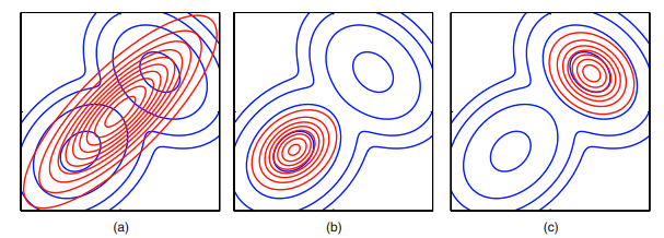
Figure 2: Possible outcomes trying to match a multimodal Gaussian with a single Gaussian. (a) shows the result of a forward-KL optimization. (b) and (c) possible reverse KL results (depends on initialization). (Image from Bishop)

Hypothesis Testing

p-value

Probability of observing a result at least as extreme as the ones obtained assuming $\mathcal{H}_0$ is correct.
Gives a metric of how likely it is to have observed something “by chance”.
If $p_{val}$ is very small $\rightarrow$ it is very unlikely to have observed what we observed under $\mathcal{H}_0$ $\rightarrow$ must be rejected (it is probably wrong as our observation is very strange).

Statistical testing pipeline

Statistical testing is used to know whether an hypothesis is significant. The main steps are as follows:

Define a null Hypothesis $H_0$ which will be rejected or not.
Define a confidence $c$ or critical value $\alpha = 1 - c$.
- If $p_{val} < \alpha \rightarrow \text{Reject hypothesis}$
- If $p_{val} > \alpha \rightarrow \text{Do NOT reject hypothesis}$
Determine the distribution our data follows.
Compute a suited test-statistic and p-value.
Reject/Don’t reject hypothesis

Common tests: z-test, t-test, ANOVA, $\chi^2$-test…

Probability Basics for ML