Ensemble Distribution Distillation $(EnD^2)$
Idea
Until recently ANNs were unable to provide reliable measures of their prediction uncertainty, which often suffer from over-confidence. Model ensembles can yield improvements both in accuracy and uncertainty estimations. Their higher computational costs motivates their distillation into a single network. While accuracy performance is usually kept after distillation, the information on the diversity of the ensemble (different types of uncertainty) is lost.
This paper presents a way to distill an ensemble of models while maintaining the learned uncertainty.
Understanding uncertainty
- Knowledge/epistemic uncertainty: Uncertainty given by a lack of understanding of the model. For instance: when an out-of distribution point or a point from a sparse region in the dataset is being assessed. Can be fixed by training with more data from those regions.
- Data/aleatoric uncertainty: Irreducible uncertainty by the data itself. For instance: because of the complexity, multi-modality or noise in the data.
- Total uncertainty: Sum of knowledge and data uncertainties.
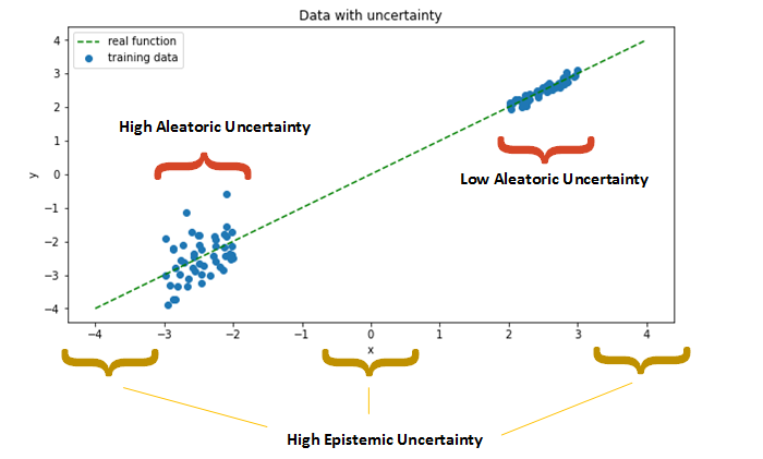
Figure 1: Types of uncertainty.
Uncertainty from an ensemble
Consider an ensemble of M models in a k-classes classification task: \(\hat{\mathcal{M}} = \left\{\mathcal{M}_1, ..., \mathcal{M}_M \right\}\) with parameters: \(\hat{\theta} = \left\{\theta_1, ..., \theta_M \right\}\). Where \(\theta_m\) can be seen as a sample from some underlying parameter distribution: \(\theta_m \sim p(\theta \mid \mathcal{D})\).
Consider now the categorical distribution which the m-th model of the ensemble yields when a data-point \(x^\star\) is evaluated: \(\pi_m = \left[ P(y=y_1 \mid x^\star , \theta_m), ..., P(y=y_1 \mid x^\star , \theta_m) \right]\). I.e. \(\mathcal{M}_m(x^\star) = \pi_m\).
From these categorical distributions (\(\pi_m\)) we can see the sources of uncertainty of our ensemble. \(\pi_m\) can be understood as the barycentric coordinates in a k-dimensional simplex. Each corner of the simplex represents a different class in the classification task. Geometrically, the probability of \(\pi\) being a particular class is given by its distance to that particular corner. For instance, in a 3-class classification problem, we can observe the following behaviors:
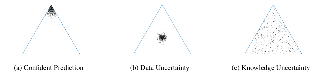
Figure 2: Representation of different uncertainties of an ensemble when evaluated on a test data-point in a 3-class task. In (a) all model predictions are close to the same corner (class), meaning all models agree. In (b) all models agree but are uncertain about which class the data-point belongs to, this happens for in-distribution uncertain samples (data uncertainty). In (c) all models disagree, some being confident about different things, a symptom of an out-of distribution input.
The closer to the simplex center a \(\pi_m\) distribution is, the higher the entropy \(\mathcal{H}\) of that distribution (more uncertainty).
This interpretation helps us understand the following identities:
-
Expected data uncertainty: \(E_{p(\theta \mid \mathcal{D})} \left[ \mathcal{H} \left[ P(y \mid x^\star, \theta )\right] \right]\). That is: the average of entropies each model of the ensemble has.
-
Total uncertainty: \(\mathcal{H} \left[ E_{p(\theta \mid \mathcal{D})} \left[ P(y \mid x^\star, \theta)\right] \right]\) That is: the spread or “disagreement” between models in the ensemble. I.e. the entropy of the average of the predictions.
Therefore, from the ensemble we can infer the model uncertainty \(\mathcal{MI}\) as:
\begin{equation} \mathcal{MI} \left[ y, \theta \mid x^\star, \mathcal{D} \right] = \mathcal{H} \left[ E_{p(\theta \mid \mathcal{D})} \left[ P(y \mid x^\star, \theta)\right] \right] - E_{p(\theta \mid \mathcal{D})} \left[ \mathcal{H} \left[ P(y \mid x^\star, \theta )\right] \right] \end{equation}
Ensemble distribution distillation
In order to maintain both the predictive accuracy and diversity of the ensemble the authors use prior networks. Prior networks: \(p(\pi \mid x; \phi)\) model a distribution over categorical output distributions \(\left( \{\pi_m \}_m \right)\). The Dirichlet distribution is chosen for its tractable analytic properties (allows closed-form expressions):
\begin{equation} p(\pi \mid x; \hat \phi) = Dir (\pi \mid \hat \alpha) \end{equation}
Where \(\hat \alpha\) is the concentration parameters vector: \(\hat \alpha_c > 0, \hat \alpha_0 = \sum_{c=1}^k \hat \alpha_c\). And \(\hat \phi\) are the set of parameters which map each input data-point \(x\) to its associated concentration parameters \(\hat \alpha\): \(\hat \alpha = f (x; \hat \phi)\). This parameters can be fitted using MLE on a dataset with all input and output of each network of the ensemble: \(\mathcal{D_e} = \left\{ x_i \pi_{i, 1:M} \right\}_{i=1}^N \sim \hat p (x \mid \pi)\). To do so, we simply minimize the following loss:
\begin{equation} \mathcal{L} \left(\phi, \mathcal{D_e} \right) = - E_{p(x)} \left[ E_{\hat p (\pi \mid x)} \left[ \log p (\pi \mid x ; \phi) \right] \right] \end{equation}
Which means (if my interpretation is not mistaken) that we get the parameters as:
\begin{equation} \phi^\star = \arg \min_\phi - \sum_{(x_i, \pi_{i, j}) \in \mathcal{D_e}} \log p(\pi_{i, j} \mid x_i, \phi) \end{equation}
Often training output distributions will be very sharp on a corner of the simplex (as in figure 2.a). Nevertheless, the initial parameters of the Dirichlet distribution are closer to the center of the simplex (assume unknown). Training with this disparity can be challenging and authors introduce a temperature annealing schedule. They “heat” or “move” first optimization steps to make the distributions more uncertain and then gradually decrease this temperature.
Results
Artificial Data
The experimented on generating the following two datasets:
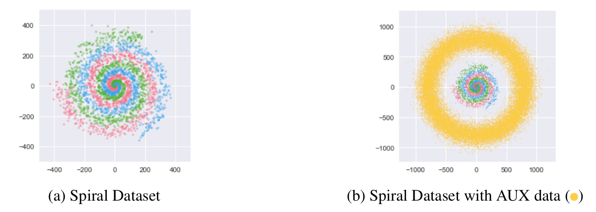
Figure 3: Artificial datasets.
Then train and assess the uncertainty of:
- 100 ANN ensemble on the first dataset (with different seeds). Classification Error: \(12.37\%\)
- Distillation into a single model of this ensemble. Classification Error: \(12.47\%\)
- Distillation of an ensemble trained also considering the \(Aux\) data. Classification Error: \(12.50\%\)
For reference, a single network had an error of \(13.21\%\)
We can visualize the uncertainty sources in the following plots:
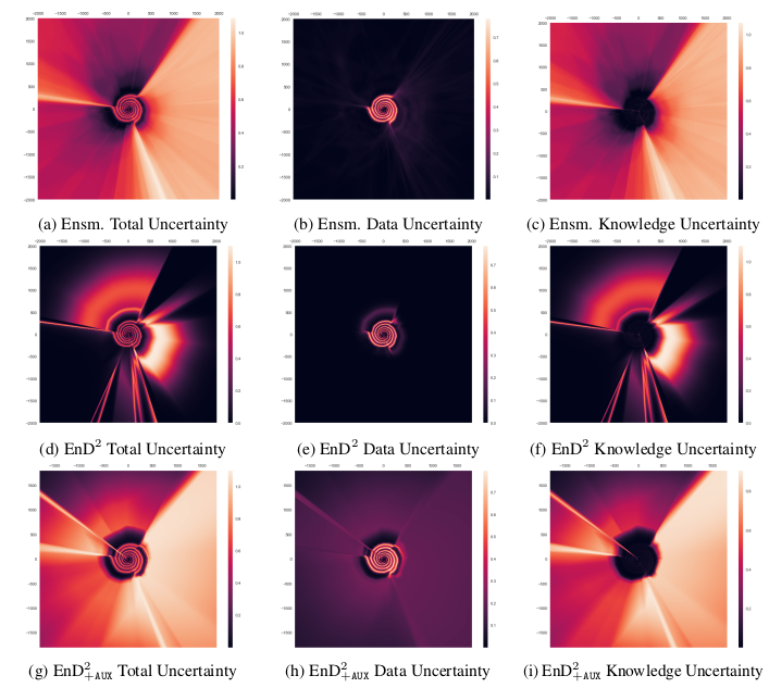
Figure 4: Artificial datasets. Notice the high data uncertainty around the spiral edges (between classes). Furthermore notice the high model uncertainty for points far away from the training sets.
To overcome that issue, the researchers sample the \(Aux\) data-points and label them with the ensemble guesses. Then use these predictions (in combination with the previous ones) to re-train the distilled model, overcoming the issue.
Without the \(Aux\) data the distilled model fails to capture knowledge uncertainty (dark areas).
Image Data
They then run similar tests on CIFAR-10, CIFAR-100 and TIM datasets reaching the following conclusions:
- Both ensemble distillation \((EnD)\) and ensemble distribution distillation \((EnD^2)\) retain the predictive performance of the ensemble.
- Both \((EnD)\) and \((EnD^2)\) show minor calibration gains w.r.t a single ANN (measured with NLL).
- When \(Aux\) data is used, \((EnD^2)\) is able to perform on par with the ensemble on a out-of-domain (OOD) detection task. Meaning it learns the ensemble behavior on unseen data.
- Image data contains a low degree of data uncertainty.
Contribution
- Novel task of distilling an ensemble into a single model maintaining the uncertainty information and diversity.
Weaknesses
- Not applied to regression tasks.
- Need of auxiliary training data to correctly assess the ensemble knowledge uncertainty.
- Need of further investigation on the temperature annealing properties process.
- Choosing a Dirichlet distribution might be too limiting: The ensemble outputs could follow a different distribution, as hinted by figure 5, where we can induce that the ensemble follows a different distribution from \((EnD^2)\). (e.g. multimodal or crescent-shaped)
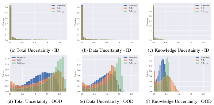
Figure 5: Histograms of uncertainty of the CIFAR-10 ensemble, EnD 2 and EnD 2+AUX on in-domain (ID) and test out-of-domain (OOD) data.