Weight Uncertainty in Neural Networks
Idea
Problem: Feed forward ANNs are prone to overfit and cannot correctly assess the uncertainty in the data. This work proposes replacing the usage of fixed weights by probability distributions over the possible values:
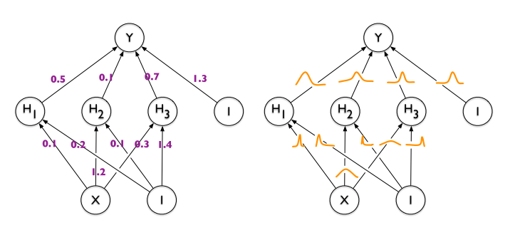
Figure 1: On the left: classic single-valued weights approach. On the right: weights as probability distribution idea.
Each weight distribution encodes the uncertainty of that connection: A network with high-variance weights implies a highly uncertain model. This leads into a higher regularization by model averaging.
By just encoding each weight distribution with 2 parameters you can train an infinite ensemble of networks from which to sample from.
How do you train this?
The authors name the training method “Bayesian by Backpropagation”. Usually ANNs weights are optimized by Maximum Likelihood Estimation (MLE):
\begin{equation} w^{MLE} = \arg \max_w \log P \left( \mathcal{D} | w \right) \end{equation}
Nevertheless, regularization can be introduced by using the Maximum A Posteriori (MAP) framework:
\begin{equation} w^{MAP} = \arg \max_w \log P \left( w | \mathcal{D} \right) = \arg \max_w \log P \left( \mathcal{D} | w \right) + \log P(w) \end{equation}
Bayesian by Backpropagation learns the MAP weights given some prior distribution. Notice that \(P ( w | \mathcal{D} )\) fully determines unseen data predictions. One can get it by marginalizing over all the network weights: \(P \left( y | x \right) = E_{P(w | D)} \left[ P \left( y | x, w \right) \right]\) (intractable in practice).
The paper proposes learning the parameters \(\theta\) of the weights distribution \(q(w \mid \theta)\) using Variational Inference. I.e. minimizing KL divergence between this \(q(w \mid \theta)\) and the true Bayesian posterior of the weights:
\begin{equation} \label{eq:vi_opt} \theta^\star = \arg \min_\theta KL \left[ q(w | \theta) \mid \mid P (w | \mathcal{D})\right] = \arg \min_\theta KL \left[ q(w | \theta) \mid \mid P (w) \right] - E_{q(w | \theta)} \left[ \log P(\mathcal{D} | w) \right] \end{equation}
Notice the trade-off between satisfying the simplicity of \(P(w)\) vs satisfying the complexity of \(\mathcal{D}\).
The optimization can be done using unbiased Monte Carlo gradients. Which means to approximate the expectations in eq. \ref{eq:vi_opt} using Monte Carlo sampling:
\begin{equation} \label{eq:vi_opt_approx} \theta^\star \simeq \arg \min_\theta \sum_i \log q(w^i | \theta) - \log p(w^i) - P(\mathcal{D} | w^i) \end{equation}
Where \(w^i\) denotes the \(i\)-th Monte Carlo sample drawn from the variational posterior \(q(w^i \mid \theta)\).
Not using a closed-form in the optimization allows any combination of prior and variational posterior. Results show similar performance between closed and open forms.
For instance, we can assume all weights follow an independent Gaussian. In this case \(\theta\) will be the vector of \(\mu, \sigma\) of each weight. The algorithm would look like this:
- Sample \(\epsilon \sim \mathcal{N} (0, I)\).
- Let \(w = \mu + \sigma \circ \epsilon\). (\(\circ\) denotes the Hadamard or element-wise product)
- Let \(\theta = (\mu, \sigma)\).
- Let \(f(w, \theta) = \log q(w \mid \theta) - \log P(w) P(\mathcal{D} \mid w)\).
- Compute gradients wrt to each parameter: \(\Delta_\mu = \frac{\partial f}{\partial w} + \frac{\partial f}{\partial \mu}\), \(\Delta_\sigma = \frac{\partial f}{\partial w} \frac{\epsilon}{\sigma} + \frac{\partial f}{\partial \sigma}\).
- Update variational parameters: \(\mu \leftarrow \mu - \alpha \Delta_\mu\), \(\sigma \leftarrow \sigma - \alpha \Delta_\sigma\).
- Go to \(1.\) until convergence.
\(\frac{\partial f}{\partial w}\) is shared between both optimizations and is the Network gradient as computed by the usual BackProp Algorithm.
The paper proposes the \(P(w)\) prior to be a combination of 2 scale mixture of normals with 0 mean. It combines one with small variance and one with a large one to make the prior more amenable during optimization.
Results
-
Performance on a simple 2-Dense layer NN is similar to the one achieved by a network of same size fitted with SGD + Dropout in the MNIST classification task.
-
Model performs well after strong (\(95\%\)) weight pruning: The scale mixture prior encourages a wide spread of the weight, translating onto a less impactful pruning.
-
Uncertainty is better estimated in regression tasks far from dataset points, where ANNs tend to be overconfident.
Contribution
-
Randomized weights improve generalisation in non-linear regression problems: Learnt representations must be robust under perturbation.
-
Weight uncertainty can be used to drive the exploration-exploitation trade-off in reinforcement learning (more systematic exploration rather than \(\epsilon\)-greedy). Weights with greater uncertainty introduce more variability into the decisions made by the network, leading naturally to exploration, as the environment is understood they become more deterministic.
Weaknesses
-
Having to optimize twice as many parameters and seeing that the results are not significantly better one could argue whether just having a network twice as big would be simpler.
-
Seems very dependent on the priors one chooses for the parameters: \(P(w)\)