In this post we talk about Latent Variable Models, and how to approximate any multimodal distribution using Variational Inference. For some motivation on why these techniques are interesting check out our Why generative models? post.
It is often the case that data \(\mathcal{D} = \{x_1, ..., x_N\}\) is distributed accordingly to some variables that cannot be directly observed (referred as latent variables \(z\)). One schoolbook examples is the Gaussian Mixture:
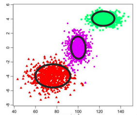
Gaussian Mixture
The likelihood of a datapoint \(x\) is given by the marginalization over the possible values of a latent variable \(z \in \{1, 2, 3\}\) that indicates the cluster.
\[p(x) = \sum_{i=1}^3 p(x\vert z=i)p(z=i)\]Latent Variable Models (LVM)
Usually though, modelling distributions with low-range discrete latent variables is not good enough. The general formula of a Latent Variable Model with a latent variable \(z\) is obtained by marginalization:
\begin{equation} \label{eq:lvm} p(x) = \int p(x \vert z) p(z) dz \end{equation}
and for a conditioned latent variable model we have:
\begin{equation} \label{eq:lvm_cond} p(y \vert x) = \int p(y \vert x, z)p(z) dz \end{equation}
This is usually the case when modelling distributions with ANNs, given \(x\), one wants to know \(p(y \mid x)\). Which can be explained by marginalizing over some simpler distribution \(z\).
Dealing with these integrals in practice is not easy at all, as for many complex distributions they can be hard or impossible to compute. In this lecture we will learn how to approximate them.
If we want to represent a really complex distribution, we can represent \(p(x \vert z)\) with a Neural Network that, given \(z\), will output the mean and variance of a Gaussian distribution for \(x\):
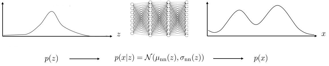
Neural Network mapping $z$ to $p(x\vert z)$
You can imagine this as a mixture of infinite Gaussians: For every possible value of \(z\), a Gaussian \(\mathcal{N}(\mu_{nn}(z), \sigma_{nn}(z))\) is summed to the approximation of \(p(x)\).
Note that \(p(x\vert z)\) is a Gaussian, but the mean and variance of this Gaussian are given by the non-linear function of the Neural Network, and therefore it can approximate any distribution.
How do you train latent variable models?
So, given a dataset \(\mathcal{D} = \left\{ x_1, x_2, \: ... \:x_N\right\}\) we want to learn its underlying distribution \(p(x)\). Since we are using latent variable models, we suspect there exists some simpler distribution \(z\) (usually Gaussian) which can be used to explain \(p(x)\).
For further motivations on why one would want to learn \(p(x)\) check out our post: Why generative models?
One can parametrize \(p(x \mid z)\) with some function \(p_\theta (x \mid z)\) and find the parameters \(\theta\) which minimizes the distance between the two. The Maximum Likelihood fit of \(p_{\theta}(x)\) finds the parameters \(\theta\) which better explain the data. I.e. the \(\theta\) which give a higher probability to the given dataset:
\begin{equation} \label{eq:ml_lvm} \theta \leftarrow \arg\max_{\theta} \frac{1}{N}\sum_{i=1}^N \log p_{\theta}(x_i) = \arg\max_{\theta} \frac{1}{N}\sum_{i=1}^N \log \left(\int p_{\theta}(x_i \vert z)p(z)dz\right) \end{equation}
The integral makes the computation intractable, therefore we need to resort to other ways of computing the log likelihood.
Why do we maximize the probability of each data-point? Our dataset is composed by samples of \(p(x)\), and we want the samples to be very likely, thus we maximize their probability. This is the essence of MLE
Estimating the log likelihood
Expectation Maximization (EM)
Eq. \(\ref{eq:ml_lvm}\) requires us to compute \(p_{\theta}(x)\), which involves integrating the latent variables (usually multi-dimensional) and is therefore intractable. Lets try to develop a bit the expression and see if we can simplify it somehow.
Turns out that by applying Jensen’s inequality on the expectation we get that for any distribution \(q(z)\):
\begin{equation} \log p_\theta(x) \ge \overbrace{E_{z \sim q(z)} \left[ \log \frac{p_\theta (x, z)}{q(z)} \right]}^{\text{Lower Bound:} \mathcal{L} (q, \theta)} = E_{z \sim q(z)} \left[ \log p_\theta (x, z) \right] - \mathcal{H} (q) \end{equation}
Things to note:
-
We say: \(\mathcal{L}(q(z), \theta) := E_{z \sim q(z)} \left[ \log \frac{p_\theta (x, z)}{q(z)} \right]\) is a lower bound of \(\log p_{\theta}(X)\)
-
Thus, by maximizing \(\mathcal{L}(q(z), \theta)\) you will also push up \(\log p_{\theta} (x)\)
-
Notice that if maximizing \(\mathcal{L}(q(z), \theta)\) wrt \(\theta\), we can just maximize \(E_{z \sim q(z)} \left[ \log p_\theta (x, z) \right]\) since \(\mathcal{H} (q)\) does not depend on it.
In essence, we are just saying that the log-likelihood of a datapoint is greater than the average of likelihoods weighted by some distribution over latent variables.
In fact:
\begin{equation} \log p_{\theta} (x) = \mathcal{L}(q(z), \theta) + D_{KL} \left(q(z) \Vert p_{\theta} (z \mid x) \right) \end{equation}
Things to note:
-
By definition: \(D_{KL} \left(q(z) \Vert p_{\theta} (z \mid x) \right) \ge 0\)
-
And \(D_{KL} \left(q(z) \Vert p_{\theta}(z \mid x) \right) = 0 \iff q(z) = p_{\theta} (z \mid x)\),
-
\(\log p_{\theta} (x)\) does not depend on \(q(z)\), so apart from maximizing \(\mathcal{L}(q(z), \theta)\) wrt \(\theta\), we can also maximize it by setting: \(q(z) \leftarrow p_{\theta} (z \mid x)\)
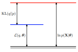
C. Bishop shows this decomposition with this figure. He represents $p(z)$ as $q$.
See chapter 9 of C. Bishop, Pattern Recognition and Machine Learning
Problem
We can maximize \(\mathcal{L}(q(z), \theta)\) wrt 2 things: \(\theta\) and \(q(z)\). But they form a cyclic dependence!!!
-
To optimize over \(\theta\), we need \(q(z)\)
-
To compute \(q(z)\) we need \(\theta\)
EM Algorithm
Expectation Maximization assumes \(p_{\theta}(z \vert x_i)\) is tractable and exploits the lower bound inequality by iteratively alternating between the following steps:
Repeat until convergence:
- E step: Compute the posterior \(q(z) \leftarrow p_{\theta^{old}}(z \vert x_i)\)
- M step: Maximize wrt \(\theta\): \(\theta \leftarrow \arg \max_\theta E_{z \sim q(z)} \Big[ \log p_{\theta}(x_i, z) \Big]\)
To solve these kind of dependencies we can iterate until convergence:
- Randomly guess \(\theta^1\)
- Use \(\theta^1\) to compute \(q(z) \leftarrow p_{\theta^1} (z \mid x)\) (expectation)
- Use \(q(z)\) to compute the \(\theta^2\) which maximize \(\mathcal{L}(q(z), \theta)\) (maximization)
- Use \(\theta^2\) to compute \(q(z) \leftarrow p_{\theta^2} (z \mid x)\) (expectation)
- …
And this is exactly what EM does!
Eq. \ref{eq:ml_lvm} then becomes the maximization of \(\mathcal{L}(q(z), \theta)\): \begin{equation} \label{eq:ml_lvm_em} \theta \leftarrow \arg\max_{\theta} \frac{1}{N}\sum_{i=1}^N E_{z \sim p(z \vert x_i)} \left[ \log p_{\theta}(x_i, z) \right] \end{equation}
EM is just fancier k-means
Its nice to notice that EM algorithm shares a similar structure to k-means clustering:
K-means: Repeats these two steps until convergence:
- Step 1: Hard assign each point (\(x_i\)) to a cluster (\(z_i\)). Should we say the expected cluster?
- Step 2: Move the cluster centroids to better fit their assigned points. Should we say maximize cluster likelihood?
EM: Repeats these two steps until convergence:
- Step 1: Soft assign each point (\(x_i\)) to a “cluster” (\(z_i\)). (Compute \(p_{\theta^{old}}(z \vert x_i)\))
- Step 2: Update “cluster” parameters to better fit their assigned points. (Maximize Lower Bound using MLE)
Things to notice:
-
k-means is restricted to spheric clusters and EM presents the flexibility of the chosen distribution. Clustering with Gaussian Mixture Model (GMM) is quite frequent: Each cluster is a Gaussian distribution.
-
If in EM we are using a discrete latent vars \(z_j\), we can imagine that instead of hard-assigning a single value to a “cluster”, we assign a probability.
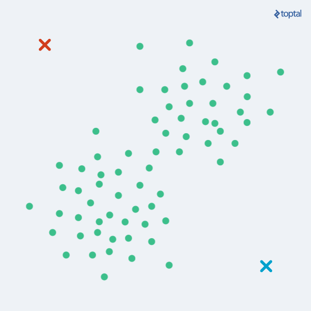
K-means example
EM on GMM example
Problems
While for discrete \(z\) values (clusters of data) computing \(p(z \vert x_i)\) might be tractable, this is not usually the case when mapping from continuous \(z\) to continuous \(p(x)\). Instead, we approximate \(p(z \vert x_i)\) with a simpler parametrized distribution \(q_i(z)\) using Variational Inference.
Variational Inference (VI)
As we said, we are interested in the maximization of Eq. \ref{eq:ml_lvm_em}, but \(p(z\vert x_i)\) is intractable. Variational inference approximates it using a tractable parametrization \(q_i(z) \simeq p(z\vert x_i)\) dependent on \(\phi_i\).
We thus have to optimize two sets of parameters:
-
\(\theta\) to parametrize the likelihood: \(p_{\theta}(x_i\vert z)\)
-
\(\{ \phi_i \}_i\) to parametrize the variational: \(q_i(z) \simeq p_{\theta}(z \vert x_i)\)
Optimizing \(\theta\)
As we show in Annex 13: Variational Inference, the log of \(p(x)\) is bounded by:
For a deeper explanation see Chapter 10.1 of C. Bishop, Pattern Recognition and Machine Learning
\begin{align}
\begin{split}
\log p(x_i) \ge & E_{z \sim q_i(z)} \Big[\overbrace{\log p_{\theta}(x_i\vert z)+\log p(z)}
^{\log p(x_i, z)}\Big]+
\mathcal{H}(q_i) \\
=: & \mathcal{L}_i(p, q_i)
\end{split}
\label{eq:elbo}
\end{align}
Where:
- \(\mathcal{H}(q_i)\) is the entropy of \(q_i\).
Things to note:
-
Again, we have that: \(\log p(x_i) \ge \mathcal{L}_i(p, q_i)\)
-
Thus, \(\mathcal{L}_i(p, q_i)\) is called the Evidence Lower Bound (shortened as ELBO).
-
Again, if you maximize this lower bound you will also push up the entire log-likelihood.
See our Information Theory Post for a better interpretation of Entropy \(\mathcal{H}\) and KL Divergence. (which we do not have access to).
Our goal is therefore to find \(\theta^*\) such that \(\mathcal{L}_i(p, q_i)\) is maximized:
\begin{equation} \theta^* = \arg\max_{\theta} \frac{1}{N}\sum_{i=1}^N E_{z \sim q_i(z)} \Big[\log p_{\theta}(x_i\vert z)+\log p(z) \Big]+ \mathcal{H}(q_i) \end{equation}
Optimizing \(\{\phi_i\}_i\)
Notice that you can also express \(p(x_i)\) as:
\begin{equation} \label{eq:dkl} \log p(x_i) = D_{KL}(q_i(z) \vert\vert p(z \vert x_i)) + \mathcal{L}_i(p, q_i) \end{equation}
Where, we can see how minimizing \(D_{KL}\) is analogous to maximizing the ELBO: We are looking to make \(q_i\) as close as possible to the real \(p(z \mid x_i)\), which will make \(D_{KL}\) smaller and the ELBO bigger.
Therefore, apart from maximizing the ELBO wrt \(\theta\) we should also maximize it wrt \(\phi_i\).
VI algorithm
VI combines both optimizations in the following algorithm:
For each \(x_i\) (or minibatch):
- Sample \(z \sim q_i(z)\)
- Compute \(\nabla_{\theta}\mathcal{L}_i(p, q_i) \approx \nabla_{\theta}\log p_{\theta}(x_i \vert z)\).
- \(\theta \leftarrow \theta + \alpha \nabla_{\theta}\mathcal{L}_i(p, q_i)\)
- Update \(q_i\) to maximize \(\mathcal{L}_i(p, q_i)\) (Can be done using gradient descent on each \(\phi_i\))
Why \(\nabla_{\theta}\mathcal{L}_i(p, q_i) \approx \nabla_{\theta}\log p_{\theta}(x_i \vert z)\)?
- Since we cannot compute the expectation over \(q_i(z)\), we estimate the expectation by sampling (We to this in step 1.)
- The gradient wrt. \(\theta\) acts only on the first expectation of Eq. \ref{eq:elbo} since the entropy does not depend on \(\theta\).
Things to note:
-
When we update \(\theta\) in step 3. we are performing the EM maximization of Eq. \ref{eq:ml_lvm_em} with \(p(z \vert x_i)\) approximated by \(q_i(z)\).
-
We update \(q_i\) by maximizing the ELBO \(\mathcal{L}_i(p, q_i)\), which in Eq. \ref{eq:dkl} we showed being equivalent to minimizing the KL Divergence between \(q_i(z)\) and \(p(z \vert x_i)\) and thus pushing \(q_i(z)\) closer to \(p(z\vert x_i)\).
What is the issue?
We said that \(q_i(z)\) approximates \(p(z\vert x_i)\). This means that if our dataset has \(N\) datapoints, we would need to maximize \(N\) approximate distributions \(q_i\). For any large dataset, such as those generated in Reinforcement Learning, we would end up having more parameters for the approximate distributions than in our Neural Network!
Amortized Variational Inference
Having a distribution \(q_i\) for each datapoint can lead us with an extreme number of parameters. We therefore employ another Neural Network to approximate \(p(z \vert x_i)\) with a contained number of parameters. We denote with \(\phi\) the set of parameters of this new network. This network \(q_{\phi}(z \vert x)\) will output the parameters of the distribution, for example the mean and the variance of a Gaussian: \(q_{\phi}(z \vert x) = \mathcal{N}(\mu_{\phi}(x), \sigma_{\phi}(x))\). Since mean and variance are given by the Neural Network, \(q_{\phi}\) can approximate any distribution.
“Amortized” because you use a single model (ANN) \(q_\phi\) to encode all \(q_i\) approximations.
The ELBO \(\mathcal{L}_i(p, q)\) is the same as before, with \(q_{\phi}\) instead of \(q_i\):
\begin{equation} \label{eq:amortized_elbo} \mathcal{L_i}(p, q) = E_{z \sim q_{\phi}(z \vert x_i)}\Big[\log p_{\theta}(x_i \vert z) +\log p(z) \Big] + \mathcal{H}\Big(q_{\phi}(z \vert x_i)\Big) \end{equation}
We now have two networks: \(p_{\theta}\) that learns \(p(x \vert z)\), and \(q_{\phi}\), that approximates \(p(z \vert x)\). We then modify the algorithm like this:
For each \(x_i\) (or minibatch):
- Sample \(z \sim q_{\phi}(z \vert x_i)\)
- Compute \(\nabla_{\theta}\mathcal{L}_i(p, q) \approx \nabla_{\theta}\log p_{\theta}(x_i \vert z)\)
- \(\theta \leftarrow \theta + \alpha \nabla_{\theta}\mathcal{L}_i(p, q)\)
- \(\phi \leftarrow \phi + \alpha \nabla_{\phi}\mathcal{L}_i(p, q)\)
We now need to compute the gradient of Eq. \ref{eq:amortized_elbo} with respect to \(\phi\):
\begin{equation} \nabla_{\phi}\mathcal{L_i}(p, q) = \nabla_{\phi}E_{z \sim q_{\phi}(z \vert x_i)}\Big[ \overbrace{\log p_{\theta}(x_i \vert z)+\log p(z)}^{r(x_i, z)\text{, constant in } \phi} \Big] + \nabla_{\phi}\mathcal{H}\Big(q_{\phi}(z \vert x_i)\Big) \end{equation}
While the gradient of the entropy \(\mathcal{H}\) can be computed straightforward by looking at the formula in a textbook, the gradient of the expectation is somewhat trickier: we need to take the gradient of the parameters of the distribution under which the expectation is taken. This is however exactly the same thing we do in Policy Gradient RL! (see the log gradient trick in our Policy Gradients Post). Collecting the terms that do not depend on \(\phi\) under \(r(x_i, z) := \log p_{\theta}(x_i \vert z) + \log p(z)\) we obtain:
\begin{equation} \nabla_{\phi}E_{z \sim q_{\phi}(z\vert x_i)} \left[r(x_i, z)\right] = \frac{1}{M} \sum_{j=1}^M \nabla_{\phi}\log q_{\phi}(z_j \vert x_i)r(x_i, z_j) \end{equation}
where we estimate the gradient by averaging over \(M\) samples \(z_j \sim q_{\phi}(z \vert x_i)\). We therefore obtain the gradient of \(\mathcal{L}_i(p, q)\) of Eq. \ref{eq:amortized_elbo}:
\begin{equation} \label{eq:elbo_pgradient} \boxed{ \nabla_{\phi}\mathcal{L_i}(p, q) = \frac{1}{M} \sum_{j=1}^M \nabla_{\phi}\log q_{\phi}(z_j \vert x_i)r(x_i, z_j) +\nabla_{\phi}\mathcal{H}\Big[q_{\phi}(z \vert x_i)\Big] } \end{equation}
Reducing variance: The reparametrization trick
The formula for the ELBO gradient we found suffers from the same problem of simple Policy Gradient: the high variance. Assuming the network \(q_{\phi}\) outputs a Gaussian distribution \(z \sim \mathcal{N}(\mu_{\phi}(x), \sigma_{\phi}(x))\), then \(z\) can be written as
\begin{equation} \label{eq:z_rep_trick} z = \mu_{\phi}(x) + \epsilon \sigma_{\phi}(x) \end{equation} where \(\epsilon \sim \mathcal{N}(0, 1)\). Now, the first term of Eq. \ref{eq:amortized_elbo} can be written as an expectation over the standard gaussian, and \(z\) substituted with Eq. \ref{eq:z_rep_trick}. \begin{equation} E_{z \sim q_{\phi}(z \vert x_i)}\Big[r(x_i, z)\Big] = E_{\epsilon \sim \mathcal{N(0, 1)}}\Big[r(x_i, \mu_{\phi}(x_i)+\epsilon\sigma_{\phi}(x_i))\Big] \end{equation}
Now, the parameter \(\phi\) does not appear anymore in the distribution, but rather in the optimization objective. We can therefore take the gradient approximating the expectation by sampling \(M\) values of \(\epsilon\):
\begin{equation} \nabla_{\phi} E_{\epsilon \sim \mathcal{N(0, 1)}} \Big[r(x_i, \mu_{\phi}(x_i)+\epsilon\sigma_{\phi}(x_i))\Big] = \frac{1}{M} \sum_{j=1}^M \nabla_{\phi}r(x_i, \mu_{\phi}(x_i)+\epsilon_j\sigma_{\phi}(x_i)) \end{equation}
Note that now gradient flows directly into \(r\). This improves the gradient estimation, but requires the \(q_{\phi}\) network to output a distribution that allows us to use this trick (e.g. Gaussian). In practice, this gradient has low variance, and a single sample of \(\epsilon\) is sufficient to estimate it. Using the reparametrization trick, the full gradient becomes:
\begin{equation} \label{eq:elbo_trick_gradient} \boxed{ \nabla_{\phi}\mathcal{L_i}(p, q) = \frac{1}{M} \sum_{j=1}^M \nabla_{\phi}r(x_i, \mu_{\phi}(x_i)+\epsilon_j\sigma_{\phi}(x_i)) +\nabla_{\phi}\mathcal{H}\Big[q_{\phi}(z \vert x_i)\Big] } \end{equation}
The difference between this gradient and that of Eq. \ref{eq:elbo_pgradient} is: here we are able to use the gradient of \(r\) directly, but in Eq. \ref{eq:elbo_pgradient} we rely on the gradient of \(q_{\phi}\) in order to increase the likelihood of \(x_i\) that make \(r\) large. This is the same we did in the Policy Gradients post, where we discussed why doing this leads to an high variance estimator. The figure below shows the process that from \(x_i\) gives us \(q_{\phi}(z \vert x_i)\) and \(p_{\theta}(x_i \vert z)\):
Notice this is what Variational Autoencoders do, first network being the Encoder \(p(z \mid x)\) and second network being the Decoder \(p(x \mid z)\).
A more practical form of \(\mathcal{L_i}(p, q)\)
If we look at Eq. \ref{eq:amortized_elbo}, we observe that it can be written in terms of the KL Divergence between \(q_{\phi}\) and \(p(z)\):
\begin{equation} \mathcal{L_i}(p, q) = E_{z \sim q_{\phi}(z \vert x_i)}\Big[\log p_{\theta}(x_i \vert z)\Big]+ \overbrace{ E_{z \sim q_{\phi}(z \vert x_i)}\Big[\log p(z) \Big] +\mathcal{H}\Big(q_{\phi}(z \vert x_i)\Big) }^{-D_{KL}\Big(q_{\phi}(z \vert x_i) \vert\vert p(z) \Big)} \end{equation} In practical implementations is often better to group the last two terms under the KL Divergence since we can compute it analytically -e.g. D. Kingma, M. Welling, Auto Encoding Variational Bayes-, and we can use the reparametrization trick only on the first term.
The Policy Gradient for \(\mathcal{L_i}(p, q)\) with respect to \(\phi\) then becomes: \begin{equation} \label{eq:elbo_pgradient_dkl} \boxed{ \nabla_{\phi} \mathcal{L_i}(p, q) = \frac{1}{M} \sum_{j=1}^M \nabla_{\phi}q_{\phi}(z_j \vert x_i)\log p_{\theta}(x_i \vert z_j) -\nabla_{\phi}D_{KL}\Big(q_{\phi}(z \vert x_i) \vert \vert p(z)\Big) } \end{equation}
The Reparametrized Gradient then becomes (single sample estimate): \begin{equation} \label{eq:elbo_trick_gradient_dkl} \boxed{ \nabla_{\phi} \mathcal{L_i}(p, q) = \nabla_{\phi} \log p_{\theta}(x_i \vert \mu_{\phi}(x_i) + \epsilon \sigma_{\phi}(x_i)) - \nabla_{\phi} D_{KL}\Big(q_{\phi}(z \vert x_i) \vert\vert p(z)\Big) } \end{equation}
Notice that in both Eq. \(\ref{eq:elbo_pgradient_dkl}\) and Eq. \(\ref{eq:elbo_trick_gradient_dkl}\), the first term ensures \(p(x_i)\) is large and the second ensures \(q_\phi(z \mid x_i)\) is close to the desired distribution of \(z\): \(p(z)\).
Policy Gradient Approach or Reparametrization Trick?
Policy Gradient (Eq. \ref{eq:elbo_pgradient_dkl}):
- Can handle both discrete and continuous latent variables.
- High variance, requires multiple samples and smaller learning rates.
Reparametrized Gradient (Eq. \ref{eq:elbo_trick_gradient_dkl}):
- Low variance (one sample is often enough).
- Simple to implement.
- Can handle only continuous latent variables.
Mean Field Approximation Variational Inference
Mean Field Approximation Variational Inference is another approach of VI which does not rely on assuming a functional form of the distribution and learning its parameters. Instead, attempts to learn both latent variables and parameters distributions by assuming independence between a subdivision of them.
\begin{equation} q(Z_1, … , Z_k, \Theta_1, …, \Theta_l) = \prod_i^a q(Z_i) \prod_j^b q(\Theta_j) \end{equation}
While not 100% accurate, it can significantly the expressions. If we attempt to maximize the ELBO we get that:
\begin{equation} q (Z_i) \propto E_{Z, \Theta - Z_i} \left[ \log p(X, Z, \Theta) \right] \end{equation}
Cited as:
@article{campusai2020vi,
title = "From Expectation Maximization to Variational Inference",
author = "Canal, Oleguer* and Taschin, Federico*",
journal = "https://campusai.github.io/",
year = "2020",
url = "https://campusai.github.io/ml/variational_inference"
}