In the previous lecture: Model-based RL, we where planning trajectories (stochastic open-loop), by maximizing the expected reward over a sequence of actions: \begin{equation} a_1,…,a_T = \arg \max_{a_1,…,a_T} E \left[ \sum_t r(s_t, a_t) \mid a_1,…, a_T \right] \end{equation}
Now we will build a policies capable of adapting to the situation (stochastic closed-loop), by maximizing a reward expectation:
\begin{equation} \pi = \arg \max_{\pi} E_{\tau \sim p(\tau)} \left[ \sum_t r(s_t, a_t) \right] \end{equation}
Naive approach
Backprop the \(s_{t+1}\) error into our env model prediction and the \(r_t\) error into our policy:
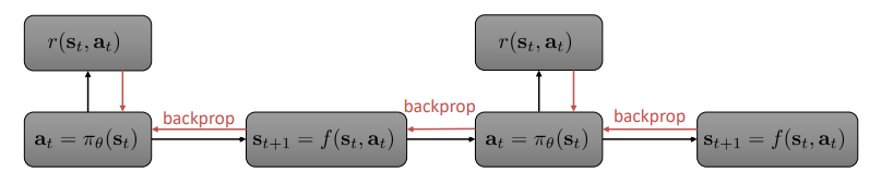
Backprop though time computational graph.
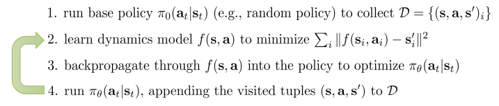
The pseudo-code would then be:
Problems:
- Propagating gradient through long trajectories often causes vanishing or exploding gradient issues (depending on the eigenvalues of the models Jacobians). But unlike LSTMs we cannot choose simpler dynamics, they are chosen by the environment.
- Ill conditioning due to high parameter sensitivity. Same as shooting methods, first actions affect trajectory much more significantly than last ones. But no dynamic programming (like LQR) can be applied since policy params couple all the time steps.
Solutions:
General idea of the solutions, developed further in subsequent sections.
-
Model-based acceleration: Use model-free RL algorithms (which are derivative free), using our learned model to generate synthetic samples. Even though it seems counter-productive it works well.
-
Use simple policies (rather than ANNs). This allows us to use second-order optimization (aka Newton Method) which mitigates the mentioned problems. Some applications are:
- Linear Quadratic Regulator with Fitted Local Models (LQR-FLM).
- Train local policies to solve simpler tasks.
- Combine them into global policies via supervised learning.
Model-free
We have two equivalent options to approximate \(\nabla_{\theta} J(\theta)\):
Policy gradient:
Avoids backprop through time as it treats the derivation of an expectation as the derivation of sums of its states probabilities:
\begin{equation} \nabla_{\theta} J(\theta) \simeq \frac{1}{N} \sum_i^N \sum_t \nabla_{\theta} \log \pi_{\theta} (a_{i, t} \mid s_{i, t}) \hat Q^\pi (s_t^i, a_t^i) \end{equation}
- Has a high variance, but can be mitigated by training with more samples: Thats where using a learned model cheaper than real env. to generate multiple synthetic samples helps.
Path-wise backprop gradient:
\begin{equation} \nabla_{\theta} J(\theta) = \sum_t \frac{dr_t}{ds_t} \prod_{t^{\prime}} \frac{ds_{t^{\prime}}}{da_{t^{\prime} - 1}} \frac{da_{t^{\prime} - 1}}{ds_{t^{\prime} - 1}} \end{equation}
- It is very ill-conditioned (unstable) since applying the chain rule to numerous successive elements of the trajectory results in the product of many Jacobians.
- If using long trajectories, our synthetic model might give erroneous estimations.
- Has a lower variance.
Dyna Algorithm
Online Q-learning algorithm performing model-free RL with a model to help compute future expectations.
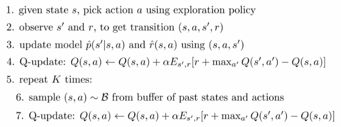
Dyna algorithm pseudocode.
We use our learned synthetic model to make better estimations of future rewards.
Generalized Dyna-style Algorithms
Online Q-learning algorithm performing model-free RL with a model to help compute future expectations.
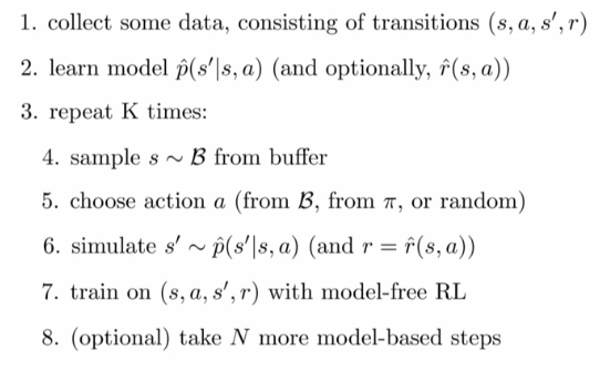
Generalyzed Dyna-style algorithms pseudocode.
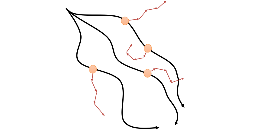
Generalyzed Dyna approach. Black arrows are the real-world traversed trajectories. Tan points the samples from which to generate synthetic trajectories. Red arrows the simulated trajectories using our learned transition model.
Pros:
- We augment the training states by generating new samples (this reduces variance).
- Env. model doesn’t need to be super good since we only use it to simulate few steps close to real states.
Cons:
- Initial env. model might be very bad and mess up the policy approximator.
- Learning a decent model of the environment in some cases might be harder than learning the Q function.
Local policies
In the standard RL setup, the main thing we lack to use LQR is: \(\frac{df}{dx_t}\), \(\frac{df}{du_t}\) (control notation).
Idea: Fit \(\frac{df}{dx_t}\), \(\frac{df}{du_t}\) around taken trajectories. By using LQR we have a linear feedback controller which can be executed in the real world.
- Run policy \(\pi\) on robot, to collect trajectories: \(\mathcal{D} = \{ \tau_i \}\).
- Fit \(A_t \simeq \frac{df}{dx_t}, B_t \simeq \frac{df}{du_t}\) in a linear synthetic dynamics model: \(f(x_t, u_t) \simeq A_t x_t + B_t u_t\) s.t. \(p(x_{t+1} \mid x_t, u_t) \sim \mathcal{N} (f(x_t, u_t), \Sigma)\).
Reminder from LQR lecture: \(\Sigma\) does not affect the answer, so no need to fit it. - Improve controller and repeat.
Controller (step 1.)
iLQR produces: \(\hat x_t, \hat u_t K_t, k_t\) s.t. \(u_t = K_t (x_t - \hat x_t) + k_t + \hat u_t\). but what controller should we execute?
- \(p(u_t \mid x_t) = \delta (u_t = \hat u_t)\) doesn’t correct for deviations or drift.
- \(p(u_t \mid x_t) = \delta (u_t = K_t (x_t - \hat x_t) + k_t + \hat u_t)\) might be so good that it doesn’t produce different enough trajectories to fit a decent env. model (you cannot do linear regression if all your points look the same).
- \(p(u_t \mid x_t) = \mathcal{N} (u_t = K_t (x_t - \hat x_t) + k_t + \hat u_t, \Sigma_t)\) adds the needed noise so not all trajectories are the same. A good choice is \(\Sigma = Q_{u_t, u_t}^{-1}\) (Q matrix from LQR method).
OBS: \(Q_{u_t, u_t}\) matrix of LQR method models the local curvature of \(Q\) function. If it’s very shallow, you can afford to be very random. Otherwise, it means that action heavily influences the outcome and you shouldn’t introduce that much variance.
Fitting dynamics (step 2.)
Ideas:
- Fit \(A_t, B_t\) matrices of \(p(x_{t+1} \mid x_t, u_t)\) at each time-step using linear regression with the \({x_t , u_t, x_{t+1}}\) point received.
Problem: Linear regression scales with the dimensionality of the state. Very high-dim states need way more samples. - Fit \(p(x_{t+1} \mid x_t, u_t)\) using Bayesian linear regression with a prior given by any global model (GP, ANN, GMM…). This improves performance with less samples.
Problem: Most real problems are not linear: Linear approximations are only good close to the traversed trajectories.
Solution: Try to keep new trajectory probability distribution \(p(\tau)\) “close” to the old one \(\hat p(\tau)\). If the distribution is close, the dynamics will be as well. By close we mean small KL divergence: \(D_{KL} (p(\tau) || \hat p(\tau)) < \epsilon\). Turns out it is very easy to do for LQR models by just modifying the reward function of the new controller to add the log-probability of the old one. More in this paper.
Still, the learned policies will be only local! We need a way to combine them:
Guided policy search
Use a weaker learner (e.g. model-based local-policy learner) to guide the learning of a more complex global policy (e.g. ANN).
For instance, if we have an environment with different possible starting states, we can cluster them and train a separate LQR controller for each cluster (each one being only responsible for a narrow region of the state-space: trajectory-centric RL). Then we can use it to learn a single ANN policy (using supervised learning) which learns starting from any state.
Problem: The learned controllers behavior might not be reproducible by a single ANN. They all have different local optima and an ANN can only have one.
Solution: After training the ANN, go back and modify the weak learners rewards to try to mimic the ANN as well.This way, after re-training, the global optima should be found:
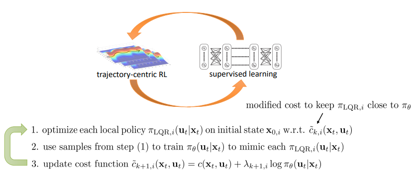
Guided policy search algorithm. $\pi_{theta}$ is the global ANN-modelled policy. $\lambda$ is the Lagrange multiplier and the sign of the equation in step 3 should be negative.
This idea of combining local policies and a single global policy ANN can be used in other settings beyond model-based RL (it also works well on model-free RL).
Distillation in Supervised Learning
Distillation: Given an ensemble of weaker models, we can train a single one that matches their performance by using each model output of the ensemble as a “soft” target (e.g. applying Softmax over them). The intuition is that the ensemble adds knowledge to the otherwise hard labels, such as: which ones can be confusing.
Policy Distillation
Distillation concept can be brought to RL. For instance in this paper they train an agent to play all Atari games. They train a different policies to play each of the games and then use supervised learning to train a single policy which plays all of them. This technique seems to be easier than multi-task RL training.
This is analogous to Guided policy search but for multi-task learning
Divide and Conquer RL
We can use the loop presented in Guided policy search also in this setting to improve the specific policies using the global policy:
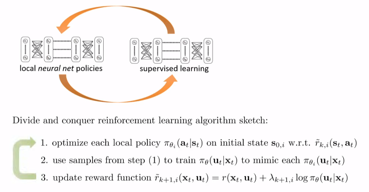
Divide and conquer RL algorithm. $\pi_{theta}$ is the global ANN-modelled policy. Now $\pi_{phi_i}$ are also modelled by ANNs. $\lambda$ is the Lagrange multiplier and the sign of the equation in step 3 should be negative. $x \equiv s$, $u \equiv a$.