Soft Actor-Critic (SAC)
Idea
Deep RL algorithms suffer from:
- High sample complexity: Most on-policy algorithms require new samples to be collected after each gradient step (too expensive in large problems).
- Brittle convergence: To solve sample complexity, off-policy algorithms aim to reuse past experience. But:
- Its not directly feasible with conventional policy gradient based methods.
- Value-based approaches (e.g. Q-learning) combined with NN give a challenge for stability (which worsens if working in continuous spaces).
To solve them, this paper implements an off-policy (deal with sample complexity), actor-critic (work in high-dim continuous spaces) algorithm in the maximum entropy framework (enhance learning robustness).
For infinte-horizon problems, a \(\gamma\) parameter can be used to make both rewards and entropies finite.
Maximum Entropy Framework
“Succeed at the task, while behaving as random as possible”: Actor aims to maximize expected reward while also maximizing entropy:
- Wider exploration discarding clearly unpromising avenues.
- Better convergence robustness as it prevents premature local optima convergence.
The optimization objective then becomes:
\begin{equation} J(\pi) = \sum_t E_{(s_t, a_t) \sim \rho_{\pi}} \left[ r(s_t, a_t) + \alpha H(\pi(\cdot | s_t)) \right] \end{equation}
Where $\alpha$ is a “temperature” meta-parameter, which can be fixed or learned ($\alpha$ = 0 for standard RL).
The Bellman (expectation) operator \(\mathcal{T}\) then becomes:
\begin{equation} \label{eq:quality} \mathcal{T}^\pi Q(s_t, a_t) = r(s_t, a_t) + \gamma E_{s+1 \sim p} \left[ V (s_{t+1}) \right] \end{equation}
Where:
\begin{equation} \label{eq:value} V (s_{t+1}) = E_{a_t \sim \pi} \left[ Q (s_t, a_t) \right] - \alpha E_{a_t \sim \pi} \left[ \log \pi (a_t | s_t) \right] \end{equation}
The value of the next state is the quality of the actions over \(\pi\) distribution at that state + the entropy of the policy at that state. Remember that the entropy of a distribution \(X\) is defined by \(H(X) = - E_x (\log(X))\).
The paper proofs the Soft policy iteration theorem. It states that the repeated application of the soft Bellman equation on a family of parametrized policies converges to the optimal one.
Algorithm
Since the algorithm lies in the Actor-Critic framework they parametrize the:
- Soft Value function: \(V_\psi\)
- Soft Q function: \(Q_\theta\)
- Tractable policy: \(\pi_\phi\)
Learning \(V_\psi\) is redundant if also learning \(Q_\theta\). Nevertheless learning both stabilizes the training process.
\(V_\psi\) is fitted to minimize the RSS with function \ref{eq:value}:
\begin{equation} \label{eq:v} J_V (\psi) = E_{s_t \sim \mathcal{D}} \left[ \frac{1}{2} \left(V_\psi (s_t) - E_{a_t \sim \pi_\phi} \left[ Q_\theta (s_t, a_t) - \log \pi_\phi (a_t | s_t) \right] \right)^2 \right] \end{equation}
\(Q_\theta\) is fitted to minimize the RSS with function \ref{eq:quality}:
\begin{equation} J_Q (\theta) = E_{s_t \sim \mathcal{D}} \left[ \frac{1}{2} \left( Q_\theta (s_t, a_t) - r(s_t, a_t) - \gamma E_{s+1 \sim p} \left[ V (s_{t+1}) \right] \right)^2 \right] \end{equation}
It has been shown that using an exponential moving average of \(\psi\) (usually referred as \(\bar{\psi}\) stabilizes training.
\(\pi_\phi\) is fitted to minimize the expected distance (KL-divergence) between a policy \(\pi \in \Pi\) (\(\Pi\) is the parameter-space we are working on), and the policy which the softmax of \(Q_\theta\) gives:
\begin{equation} \label{eq:pi} J_\pi (\phi) = E_{s_t \sim \mathcal{D}} \left[ D_{KL} \left(\pi_\phi (\cdot|s_t) \mid \mid \frac{exp( Q_{\theta} (s_t, \cdot)}{Z_\theta} \right) \right] \end{equation}
Where \(Z_\theta\) is used to normalize the exponential of \(Q\) distribution. Notice that in general it is intractable but since it does not contribute to the gradient w.r.t. the policy parameters, it can be ignored.
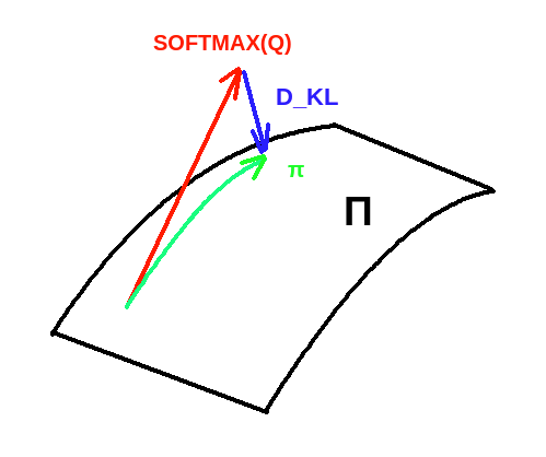
Interpretation of eq \ref{eq:pi}. We take the closest policy to SOFTMAX(Q) from our parametrized space by the KL divergence projection.
The algorithm then becomes:
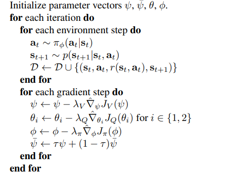
SAC algorithm.
They use 2 Q-function approximators to mitigate positive bias in policy improvement adn speed training. Eq \ref{eq:v} uses the minimum value of the 2 Q-functions.
Contribution
- Stable Learning: Results show similar performance across different seeds, in contrast to other off-policy methods.
- Better than other SOTA algorithms (DDPG, PPO, TD3) in complex environments: Maximum entropy framework improves performance in those cases.
Weaknesses
- It presents a high variability when using deterministic policies (cannot take advantage of entropy). Since SAC converges to stochastic policies, it is often beneficial to make the final one deterministic.
- Sensitive to reward scaling. Since it affects the temperature parameter controlling the entropy. Larger reward means lower entropy.