NOTE: Transfer Learning (TL) & Multi-task Learning (MTL) are still an open problem in DRL, this lecture is more a survey on latest research rather than some well-established methods.
TL Terminology:
- Task: In the RL context, task is the same as MDP.
- Source domain: Initial task where the agent has been trained.
- Target domain: Task which we want to solve. (We aim to transfer knowledge from source to target domain).
- n-shot: Number of attempts in the target domain before the agent is able to solve it. (often used as 0-shot, 1-shot or few-shot)
TL in RL
Prior understanding of problem structure can help us solve complex tasks quickly and have better performance.
Where and how can we store knowledge?
- Q-function: Remember which state-action pairs are good
- Policy: Remember which actions are useful in a given state (and which are never useful)
- Models: Remember physics laws, so you do not have to learn them again
- Features/hidden states: Re-using ANN feature extractors when re-training an agent (one of the most common uses)
In this Loss is its own Reward: Self-Supervision for Reinforcement Learning they show its effectiveness in vision-based tasks (although only in the same kind of task):
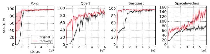
Evolutions when training a policy from scratch (black) vs using pre-trained weights for all except last layer (red). As expected using pre-trained feature extractors significantly speeds the learning process. Image by OpenAI.
This example shows the two jobs the model is doing:
- Extract features from observations.
- Extract value from these features.
By inputing extracted features, the model learns much quickly as it only needs to focus on task 2.
Forward transfer
In short: Train on one task, transfer to a new one
In supervised learning, we usually perform TL as follows:
- Train a large network in a large dataset (e.g. train a big resnet on imagenet)
- Substitute last layers of the networks for randomly-initialized ones.
- Depending on the size of our dataset:
- If small: train only updating the weights of the last new layers
- If large: train all weights
This methodology is very effective in vision tasks.
Problems:
- Domain shift: Representations learned in the source domain might not work on the target domain. Usually, we take the invariance assumption: everything that is different from both domains is irrelevant. While not usually true, if it was true, there exist some things we can do to deal with domain shift. For instance, we can train using domain confusion (aka domain-adversarial NN): Instead of updating the weights just from the main task, we can also use the reversed gradient of a classification tasks which learns to tell apart both domains from a latent representation of the input.
But, how does that idea translate into RL?
Naive approach
Train a policy on the source domain and test it on the target domain (hoping for the best). Usually does not work.
Finetuning
Train on a task, re-train on a new one using the first feature-extraction layers of the ANN (essentially the same explained before but changing tasks). It is specially useful for vision-based policies. One can even train the feature-extraction layers in a supervised learning setup with some famous dataset.
Problems:
- Too specialized policies. If the domains are too distinct weight transfer can worsen things since policies tend to become very specialized.
- Too deterministic policies. Some methods (e.g. policy gradient) favour a lot good actions while lowering the probability of the bad ones: when moved to a new domain they will not explore enough. This gets improved by using maximum-entropy policies, which try to maximize rewards while acting as randomly as possible.
Something that also improves performance is to pre-train for robustness, for instance: try to learn solving tasks in all possible ways:
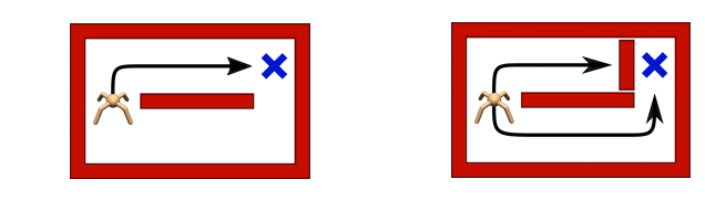
Learning multiple ways to solve first (right) maze will help should it be changed as in the second (left) image. Obtaining thus, a more robust transfer.
When finetuning we usually do not want to maximize entropy as we usually want to squeeze the best performance out of our agent. Usually in the Maximum Entropy Framework we have a temperature parameter to tune the amount of entropy desired. If the output of our ANN is a multivariate Gaussian, we can reduce its variance. Though it has not been trained that way it usually works.
Domain manipulation
If we have a very difficult target domain we can design our source domain to improve its transfer capabilities. Same idea remains: The more diversity we see, the better will the transfer be.
For instance, if training on some physical system, one can use a source domain with randomized variables (e.g. weight and sizes) to make a more robust transfer: EPOpt: Learning Robust Neural Network Policies Using Model Ensembles
Variable randomization example in hopper environment.
Other ideas, such as the ones presented in: Preparing for the Unknown: Learning a Universal Policy with Online System Identification rely on learning some physical parameters of the environment in a supervised manner in source domains, which are also feeded into the policy. Later, on the target domain they are estimated. Results show that this approach achieves almost the same performance as directly feeding the real parameters to the policy.
Some ideas explore visual randomization of the environment. For instance, in simulation, change walls textures to have a more robust policy.
More on simulation to real RL in this paper.
Domain adaptation
So far we talked about pure 0-shot transfer: Learn in source domains so we can succeed in unknown target domains, we thus needed to be as robust as possible. Nevertheless, we can usually sample some states (e.g. images) from our target domain and do something smarter than pure randomization.
Adapting Deep Visuomotor Representations with Weak Pairwise Constraints applies the domain confusion (aka adversarial domain adaptation) idea we previously presented to RL. They synthetically create simplified states in the source domain to train on. Later, they force the model to represent both synthetic and real states by the same kind of features. To do so in a vision task: you impose some loss on the higher level of the CNN which forces the extracted features of images from different domains to look similar to each other.
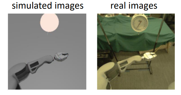
Example of a synthetic simplified state and its corresponding real one in a vision task.
A way to do this is by automatically pairing simulated images with real images and regularize the features together to get similar values.
Problem: Usually we do not have this kind of knowledge. We just have samples of both synthetic and real state extracted with some policy (e.g. random). They are not from the same state but both come from the same sampling distribution.
Solution: Use an unpaired distribution alignment loss between features (e.g. use some kind of GAN loss). You can achieve that by putting a small discriminator on the features of your network as depicted:
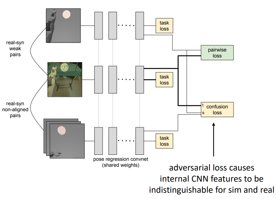
Adversarial domain adaptation network adaptation.
This other approach explicitly uses a GAN to convert the simplified state images into realistic ones in a pixel to pixel fashion. The generator gets inputed the simplified states and makes them look as similar as possible to the source domain state images. The discriminator then tries to take apart the real from the generated images. Creating thus a competition between generator and discriminator which forces the generated images to get similar to the real ones.
Multi-task transfer
In short: Train on many tasks, transfer to a new one
So far, we need to design (simulation) diverse very similar tasks to achieve a good transfer. But humans do not work this way! We transfer knowledge from multiple different tasks. This is very hard with our current algorithms, we can get what is known as negative transfer: using pre-trained weights actually harms the learning of the target task.
Transfer in Model-based RL
Even if all past tasks are different they might have things in common, for instance: the same laws of physics (e.g. same robot doing different chores / some car driving to different destinations / different tasks in same open-ended video game).
In model-based RL we can train an environment model on past tasks and use it to solve new tasks. Sometimes we’ll need to fine-tune the model for new tasks (easier than fine-tunning the policy).
Learn a multi-task policy
The idea is to learn a policy which solves multiple tasks with the hopes that:
- It will be easier to fine-tune to new tasks.
- Learning multiple tasks simu
Train single policy in a joint MDP
The most basic approach would be to construct a single MDP which describes all tasks. This MDP is composed by multiple smaller MDPs (one for each task). Then you train your policy on the big MDP, where the first state tells you in which task you are.
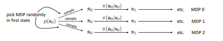
Joint MDP approach.
Example: You can train an agent to play multiple Atari games (each one having its own MDP), then in the first state you just sample one game to play.
Problems:
- Gradient interference: Becoming better at one task can make you worse at another.
- Winner-take-all problem: If a task starts getting good, the algorithm may start to prioritize that task to increase average expected reward, harming the performance of the others. (Snowball effect)
Therefore, in practice attempting this kind of multi-task RL is very challenging.
Train multiple policies in different MDPs and join them
As explained in Model-based policy learning lecture we can use distillation for multi-task transfer. Essentially, you train a policy for each of the domains you have and use supervised learning to create a single policy from the multiple learned ones.
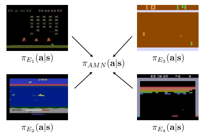
Distillation idea scheme.
We want to find the parameters which make the joint policy distribution be as close as possible to the original ones.\ Thus, we can run MLE on the following cross-entropy loss:
\begin{equation} \mathcal{L} = \sum_a \pi_i (a \mid s) \log \pi_{AMN} (a \mid s) \end{equation}
The idea is similar to Behavioral Cloning (BC lecture), but copying learned policies instead of human demonstrations.
Results show that depending on the game the transfer is beneficial or not. In particular, it is beneficial among those games which share similar traits and counterproductive in those that stand out for being different than the others.
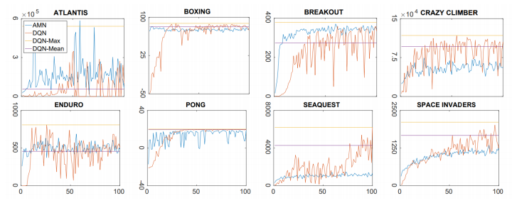
Distillation transfer results (blue) vs standard methods (red, yellow, purple).
Contextual policies
Sometimes instead of solving tasks in different environments, we need our agent to solve different tasks in the same environment. In this case we need to indicate which goal we want our agent to achieve. We can do that by adding some indication in the policy and converting it into a contextual policy:
\begin{equation} \pi_\theta (a \mid s) \rightarrow \pi_\theta (a \mid s, w) \end{equation}
Formally, this simply defines and augmented tate space \(\hat s = [ s, w ]\) where \(\hat S = S \times \Omega\), where we simply append the context.
Multi-objective RL within the same environment
It is common that we want to solve different tasks within the same environment. More formally, we have constant dynamics \(p(s_{t+1} | s_t, a_t)\) but different reward functions (one for each task). For instance, we have a kitchen robot that has to cook multiple recipes: while the setup is the same, each recipe has a different reward function associated with it.
In this case, what is the best object to transfer?
Model
If doing model-based-RL, it, should be the easiest thing to transfer, as (in principle) it is independent of the reward. While this works, it still presents some problems if attempting 0-shot transfer:
- Exploration limitations: Maybe in the source domain we only visited the subset of states which were relevant for the source task, the target task might need to use other states which the model hasn’t been trained on.
Value Function $Q$
Might be tricky since it entangles environment dynamics, policy and reward. Nevertheless, it turns out that usually these things are coupled linearly, so it is not that hard to disentangle. Introducing successor features:
These ideas are presented in Successor Features for Transfer in Reinforcement Learning
Lets remember the Bellman equation:
\begin{equation} Q^\pi (s, a) = r (s, a) + \gamma E_{s^\prime \sim p(s^\prime \mid s, a), a^\prime \sim \pi (s^\prime)} \left[ Q(s^\prime, a^\prime) \right] \end{equation}
Lets consider a vectorization of the value function: \(q = \text{vec} \left( Q^\pi (s, a) \right) \in \mathbb{R}^{\vert S \vert \cdot \vert A \vert}\). We then can linearly approximate the Bellman equation as:
\begin{equation} q = \text{vec} (r) + \gamma P^\pi q \end{equation}
Notice that if the state or action spaces are continuous this still holds for infinite-dimensional vectors.
We call \(P^\pi\) the transition probability matrix according to policy \(\pi\). Then we have that:
\begin{equation} q = (I - \gamma P^\pi )^{-1} \cdot \text{vec} (r) \end{equation}
Imagine the different tasks we want to solve have reward functions which are a linear combination of \(N\) different features: \(\text{vec} r(s, a) = \phi w\) (\(\phi\) is a matrix that encodes this relationship). We can then define a matrix \(\psi := (I - \gamma P^\pi )^{-1} \cdot \phi\). Effectively linearly disentangling the dynamics from the reward:
\begin{equation} Q^\pi = \psi w \end{equation}
We say that the i-th column of \(psi\) is a “successor feature” for the i-th column of \(\phi\). So for any linear combination \(\phi\), we can get a Q-function by applying the same combination on \(\psi\).
Notice this works on a value policy \(Q^\pi\) but it doesn’t on the optimal value function \(Q^\star\). Remember that:
\begin{equation} Q^\star (s, a) = r (s, a) + \gamma E_{s^\prime \sim p(s^\prime \mid s, a)} \left[ \max_{a^\prime} Q(s^\prime, a^\prime) \right] \end{equation}
The \(\max\) function makes the expression to be NOT linear!
How do we learn this in practice?
Simplest use: Evaluation
- Get a small amount of data of the new MDP: \(\{ (s_i, a_i, r_i, s_i^\prime)\}_i\)
- Fit \(w\) such that \(\phi (s_i, a_i) w \simeq r_i\) (e.g. with linear regression)
- Initialize \(Q^\pi (s, a) = \psi (s, a) w\)
- Finetune \(\pi\) and \(Q^\pi\) with any RL method
More sophisticated use:
- Train multiple \(\psi^{\pi_i}\) functions for different \(\pi_i\)
- Get a small amount of data of the new MDP: \(\{ (s_i, a_i, r_i, s_i^\prime)\}_i\)
- Fit \(w\) such that \(\phi (s_i, a_i) w \simeq r_i\) (e.g. with linear regression)
- Choose initial policy \(\pi (s) = \arg \max_a \max_i \psi^{\pi_i} (s, a) w\)
Notice that if the state or action spaces are continuous this still holds for infinite-dimensional vectors.
Policy
While doable with contextual policies, it might be tricky otherwise, since it contains the “least” dynamics information.
Architectures for multi-task transfer
So far we only aimed to model a policy for multiple tasks with a single ANN. But what if the tasks are fundamentally different? (e.g. they have different inputs) Can we design architectures with reusable components? (to then re-assemble them for different goals)
Introducing modular networks in deep learning (paper). They present a (quite engineered) algorithm to answer questions of a given image. They combine modules for finding text entities in images and modules to extract purpose of the question to provide an answer.
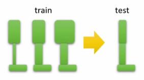
This work brings this idea to RL. In a setup with \(n\) robots working on \(m\) tasks instead of having a single ANN policy which learns to deal with any case, we can de-couple the robot control from the task goal and learn each one in a modular fashion:
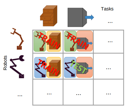
Modular ANN training approach. Different robots learn different tasks in a modular setup. Notice that you only need 2 different modules (robot and task) to learn 4 situations.
The performance of this approach depends on how many different values you have of this factors of variation and the information capacity between the modules is not too large (otherwise you need to use some kind of regularization).
Cited as:
@article{campusai2020mtrl,
title = "Transfer and Multi-Task Reinforcement Learning",
author = "Canal, Oleguer*",
journal = "https://campusai.github.io/",
year = "2020",
url = "https://campusai.github.io//rl/transfer_and_multitask_rl"
}