Neural Network Surgery in Deep Reinforcement Learning
Context
As we learned in many of our experiments, training DRL agents can be an extremely time consuming task. Specially when performing changes in the environment: As an example, in our Autonomous Driving, we often made changes to the observation space, such as changing the number of lidar rays and next visible path points. In other cases, one may want to add a new action to an agent that was previously trained. Similarly, one may want to experiment with the number of layers and nodes of the ANNs. All these changes to the network architecture require the agent to be re-trained from scratch..
In this work, taking inspiration from Neural Network Surgery with Sets, we implement a simple weight transplanting functionality that allows us to move weights from a trained network to a new network with a different architecture. We show that this simple weight transplant achieves faster and better training than re-training the new network from scratch.
Change the paradigm!
The situation in which many Deep Reinforcement Learning researchers or practitioners may find themselves into falls in the pattern:
- Choose the observation space for the given problem, the action space, the network size and parameters
- Train the agent
- Realize that the action space or the observation space was not good, the network was too big/small
- Modify the network architecture by adding/removing inputs, outputs, layers
- Train again from scratch
Our project aims to change this paradigm into
- Choose the observation space for the given problem, the action space, the network size and parameters
- Train the agent
- Realize that the action space or the observation space was not good, the network was too big/small
- Modify the network architecture by adding/removing inputs, outputs, layers
- Transplant weights from the old, trained network to the new one
- Train the new network
- Achieve faster and better training results!
Transplanting the weights
Labeling layers and units
Transplanting the weights is pretty straightforward. We use IDs to identify layers and input/output units. We then pair the ids from the old network to the new one and transfer the weights in such a way that the relations are kept as similar as possible.
Transplant
We implemented the transplant for Dense and Convolutional layers.
-
For Dense layers, a change (addition,removal or permutation) in input features’ IDs is translated into the columns of the weight matrix. Similarly, a change of output IDs is translated into the rows of weight and biases matrices. When adding new inputs or outputs, weights are left untouched from the untrained initialization.
-
For Convolutional layers, we use the same technique but inputs’ IDs refer to input channels and output IDs to the layer filters. A change (addition, removal or permutation) between the trained layer and new layer of input IDs is applied into each filter’s channel. A change of output ids is translated into the same change in the filters of the layer. This is done to maintain the operations that each input receives through the network.
Initialize the new layers
The goal is that the new architecture before starting the training behaves as close as possible to the old one.
-
Dense layers matrices are initialized as close as possible to identities, with zero biases.
-
In Convolutional layers we set the filters to be all zero but a one in top-right positions for all channels. This ensures the input and output are similar enough so the weights previously learned in posterior dense layers are not compromised.
Experiments
We performed a set of experiments to test the weight transplant performances. All the experiments have the following structure:
- Train a network to solve the problem
- Modify the network architecture
- Transplant weights to the new architecture
- Train the new architecture with the transplanted weights
- Train the new architecture initialized from scratch
- Compare results of 1, 4 and 5.
Different outputs in MNIST classification
First, we train a model to classify only MNIST images that contain digits from 0 to 3, therefore the Convolutional Neural Network has 4 outputs. Then, we transplant the weights into a new network that will classify digits from 4 to 9, and will therefore have 6 outputs. The figure below shows the training results.
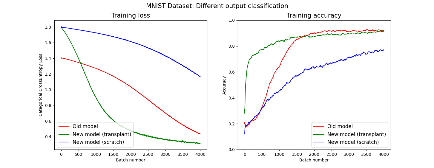
Red lines represent the old architecture, with 4 output classes. Blue lines represent the new architecture with 6 classes, trained from scratch, while green lines represent the new architecture trained starting from the transplanted weights.
Notice how the accuracy achieved by the model with transplanted weights (green) quickly rises and results in a \(\sim\) 20% improvement with respect to the same model trained from scratch (blue) in the same number of training steps. This is really interesting as the new network received weights from one that classified completely different digits.
Deep Reinforcement Learning: Cartpole environment
In the Gym Cartpole environment the goal is to balance a pole by controlling the cart on which it is attached. The observation space is \(O = (x, \dot{x}, \theta, \dot{\theta})\), i.e. position and velocity of the cart, angle and angular velocity of the pole. The cart can be controlled by, at each step, applying a force from the left or from the right. In all these experiments we use the DQN algorithm (we explained it in Lecture 8) and we perform transplants on its Q network.
Increasing the observation space
As first experiment, we train the DQN agent by pretending that the environment produced only \(\dot{x}\) and \(\theta\) as observations. The Q network has therefore 2 input units, and two output units (for the two possible actions). Then we transplant the weights into a new architecture that takes 4 inputs, and we train it on the environment with full observation space. The figure below shows the results.
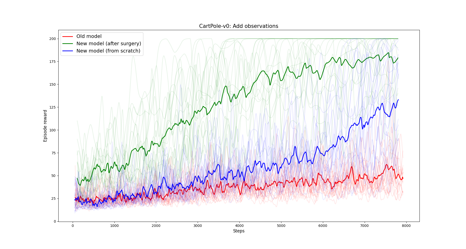
Results are averaged over 20 runs.
Notice how the Q network that received the weight transplant (green) dramatically outperforms the same architecture if initialized from scratch (blue).
NOTE: This experiment is important as it resembles a situation that happens often when working with custom environments. Often, one realizes that the agent is not learning because the observation space does not provide all the information needed. Then, modifying it, transplanting the weights and train again may be really beneficial.
Adding hidden units and layers
Another reason why an agent is not learning enough could be that the network is too small. In this experiment we train a DQN agent on the Cartpole environment on two small networks, and we apply the transplant to move the weights to two bigger networks.
- In the first figure, the Q network had two layers of 4 hidden units, and the weights are transplanted into a bigger network of 2 layers of 16 units.
- In the second figure, the Q network had a single layer of 8 units, and the weights are transplanted into a bigger network of 2 layers of 8 units. Both figures show the average of 20 DQN runs.
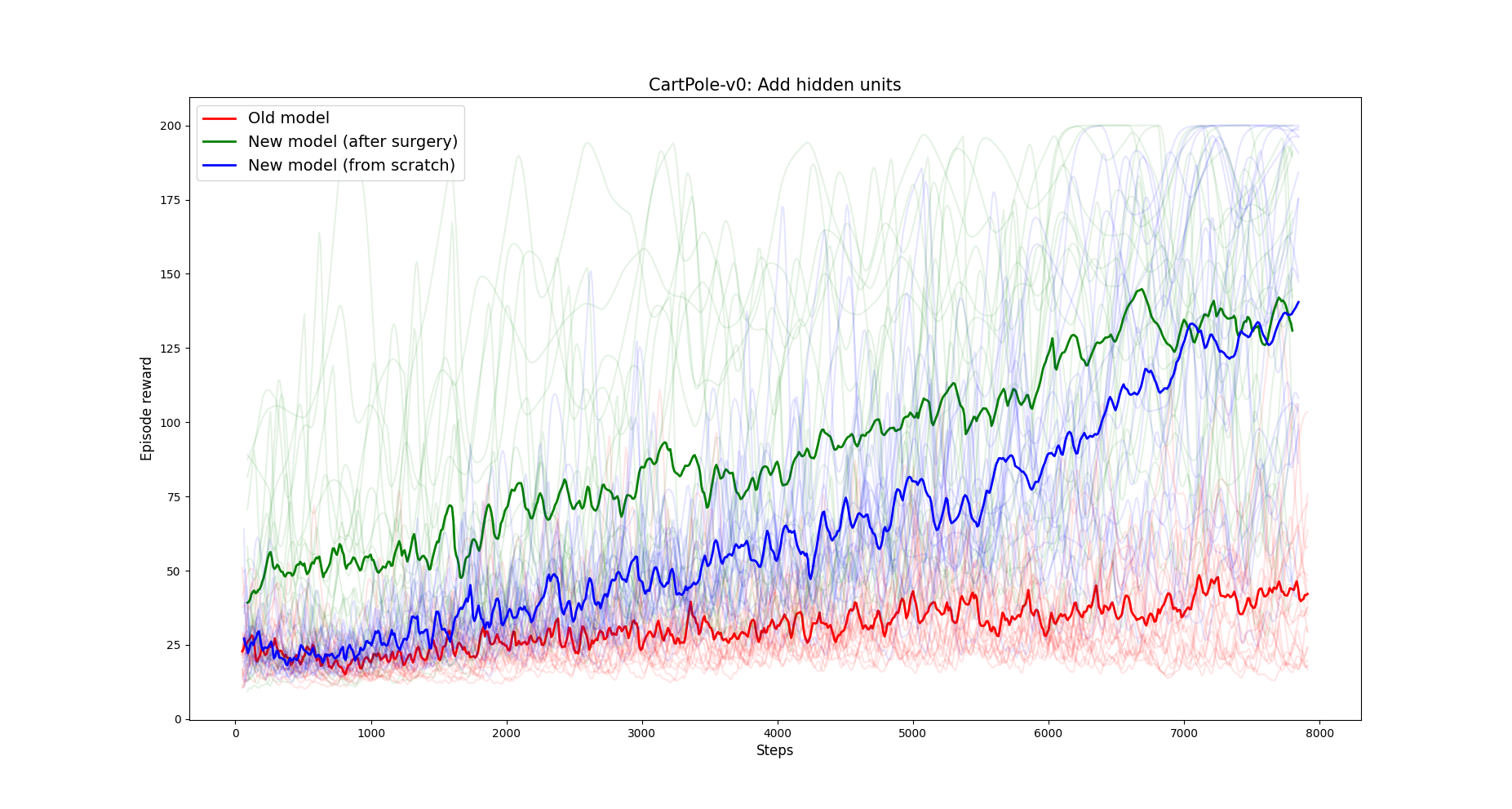
1. Adding hidden units to the Q network. In green the reward after transplanting weights, in blue the reward of the same network trained from scratch. In red the old Q network.
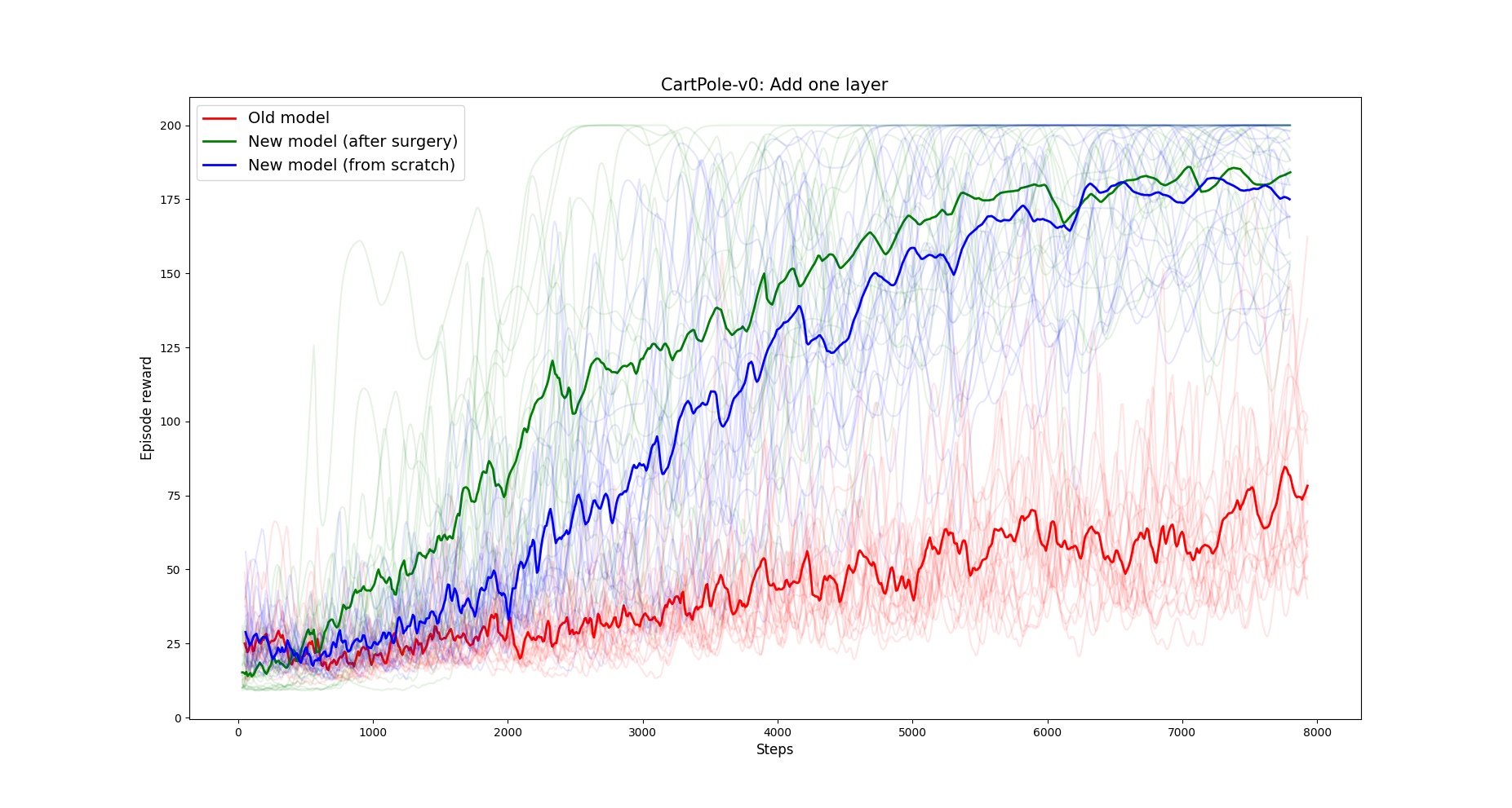
2. Adding a layer to the Q network. In green the reward after transplanting weights, in blue the reward of the same network trained from scratch. In red the old Q network.
Notice how in both cases the network that received weights with the transplant outperforms the same network trained from scratch with default initialization.
Deep Reinforcement Learning: Acrobot environment
The Acrobot environment is similar to Cartpole. The goal is to make a two joints system reach the highest possible point. The observation space is a 6-dimensional vector made of the \(\sin\) and \(\cos\) of the two angles of the two joints, and the two angular velocities. We can control it by applying a force clockwise or counter clockwise to the first joint, or do nothing.
Adding one action
The possible actions are 3, but in this experiment we first train the DQN agent by only allowing it to exert a force clockwise and do nothing. The Q network has therefore 2 output units. Then, we transplant the weights into a new network with the same architecture but with 3 output units, and we train it allowing it to perform all the three possible actions.
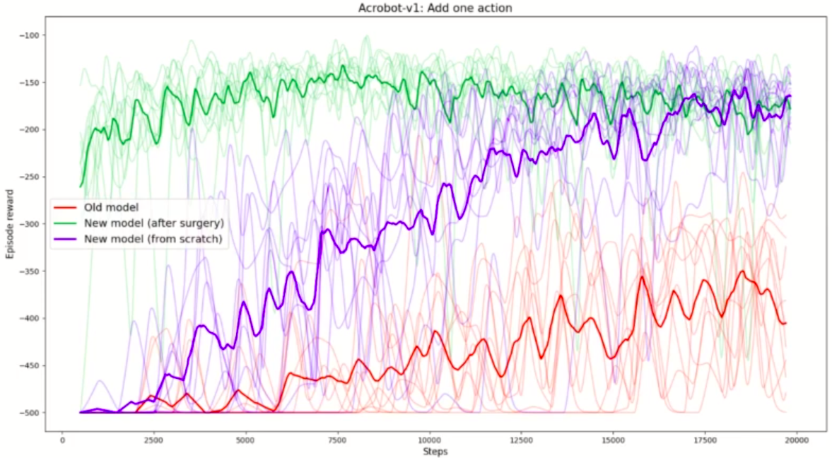
Adding an output to the Q network. Green line shows the reward for the network that received weights with transplant. The blue line is the same architecture but trained from scratch. Red line is the old architecture.
Notice that the network that received the weights with transplant starts already at high rewards, meaning that the transplant didn’t make the network forget what it learned in the old model. The network that was trained from scratch with default initialization instead takes several thousands steps to achieve the same rewards.
Deep Reinforcement Learning: Lunar Lander environmet
In the Lunar Lander environment the goal is to make the lander to land in the defined areas. Observation space is made of \(x\) and \(y\) position and velocity, angle and angular velocity of the lander. The possible actions are firing from one of the three engines or do nothing.
Adding two actions
Similar to the experiment before, we train the Q network to only perform two actions, corresponding to firing the left and right engines. Then, we transplant the weights into a new network with four outputs, corresponding to the full action space, and we train it.
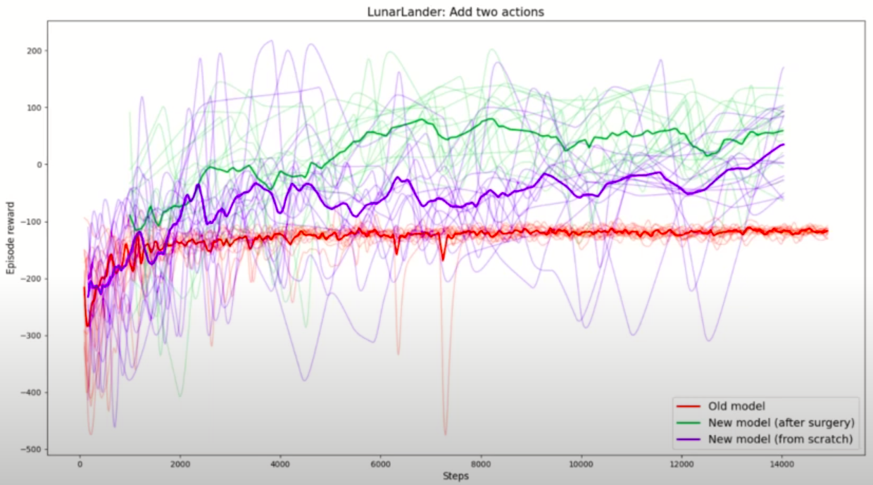
Once again, the transplant technique proved superior to training from scratch.
Future work
-
Develop a library that performs weight transplant from one network to another in different Deep Learning frameworks (Tensorflow, Pythorch) as well as for several Deep Reinforcement Learning libraries (baselines, stable-baselines, Keras-RL, etc).
-
Do more research on the initialization of new weights. Is “close-to-identity” initialization for new layers the better way? How do we initialize new output layers for Deep Reinforcement Learning value networks without destroying the policy?
-
Perform more and more complex experiments. Is the transplant always beneficial? In what cases does it fail?
Takeaways
-
Our experiments suggest that weight transplant could be really useful or Deep RL practitioners and researcher when exploring state and action space definitions, or neural network architectures.
-
Weight initialization must be done carefully in Deep Reinforcement Learning. For instance, when rewards are negative, initializing an output unit with a zero weight will make it almost always be chosen by the DQN algorithm.
-
There does not seem to be any library implementing this transfer for DRL algorithms.