Simple ML models
This post is more a memory-refresher list of simple ML models rather than a comprehensive explanation of anything in particular.
Supervised Learning
k-Nearest Neighbor (kNN)
Solves: Classification, Regression
Method: Estimate new point labels by considering only the labels of the \(k\)-closest points in the provided dataset.
Pos/Cons:
- Simplicity.
- Only one meta-parameter.
- If the dataset is very big, it can be slow to find closest point.
Characteristics: discriminative, non-parametric
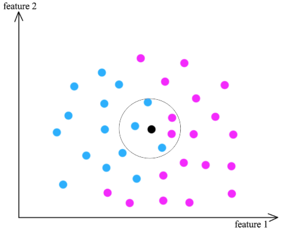
It is a good idea to choose a \(k\) different than the number of classes to avoid draws.
Decision Trees
Solves: Classification, Regression
Method: Learn decision rules based on the data features. These decisions are encoded by a tree structure where each node represents condition and its branches the possible outcomes. The conditions are chosen iteratively granting a higher information gain (the split of data which results in the lowest possible entropy entropy state).
Pos/Cons:
- Intuitive and interpretable.
- No need to pre-process the data.
- No bias (no previous assumptions on the model are made)
- Very effective, often used in winning solution in Kaggle
- High variance (results entirely depend on training data).
This high-variance issue is often addressed with variance-reduction ensemble methods. In fact, there is a technique specially tailored to decision trees called random forest: A set of different trees are trained with different subsets of data (similar idea to bagging), and also different subsets of features.
Characteristics: discriminative
Naive Bayes
Solves: Classification
Method: Given a dataset of labelled points in a \(d\)-dim space, a naive Bayes classifier approximates the probability of each class \(c_i\) of a new point \(\vec{x} = (x^1, ..., x^d)\) assuming independence on its features:
Naive because it assumes independence between features.
\begin{equation} p(\vec{x}) = p(x^1, …, x^d | C) \simeq p(x^1 | C) … p(x^d | C) \end{equation}
By applying the Bayes theorem:
\begin{equation} p(c_i \mid \vec{x}) = \frac{p(\vec{x} \mid c_i) p(c_i)}{p(\vec{x})} \simeq \frac{p(x^1 \mid c_i) … p(x^d \mid c_i) p(c_i)}{p(x^1)…p(x^d)} \end{equation}
Notice that we don’t actually need to compute the evidence (denominator) as it only acts as a normalization factor of the probabilities. It is constant throughout all classes.
We can then estimate:
- \(p(x^j \mid c_i)\) as the ratio of times \(x^j\) appears with and without \(c_i\) in the dataset.
- \(p(c_i)\) as the ratio of points classified as \(c^i\) in the dataset.
Pos/Cons:
- Simplicity, easy implementation, speed…
- Works well in high dimensions.
- Features in real world are not independent.
Characteristics: generative, non-parametric
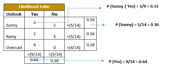
Example of how marginalization is done and independence is assumed.
Support Vector Machines (SVMs)
Solves: Binary classification
Method: Learn the hyperplane parameters which “better” split the data. It is framed as a convex optimization problem with the objective of finding the largest margin within the two classes of points. The points from each group to optimize the hyperplane position are called support vectors.
-
Maximum Margin Classifier attempts to find a “hard” boundary between the two data groups. It is however very susceptible to training outliers (high-variance problem).
-
Soft Margin approach allows for the miss-classification of points, it is more biased but better performing. Often cross-validation is used to select the support vectors which yield better results. Notice this is just a way to regularize the SVM to achieve better generality.
Schematically, SVM has this form:
\begin{equation} \vec{x} \rightarrow \text{Linear function}: \space \vec{w}^T \cdot \vec{x} \rightarrow \begin{cases} if \geq 1 \rightarrow \text{class 1} \newline if \leq -1 \rightarrow \text{class -1} \end{cases} \end{equation}
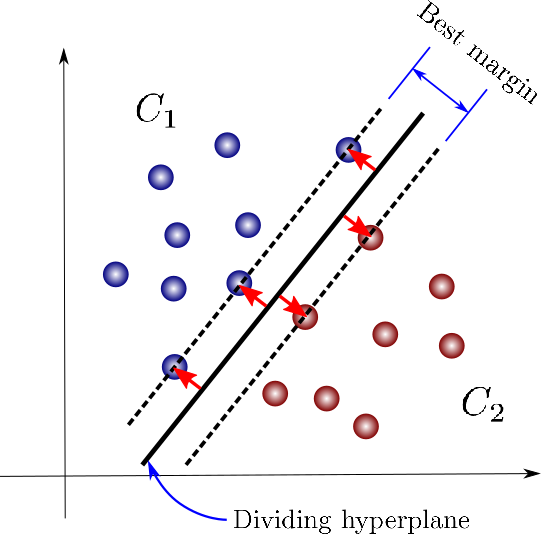
2-dim SVM.
Kernel
More often than not, the data is not linearly-separable. We can apply a non-linear transformation into a higher-dimensional space and perform the linear separation there. We call this non-linear transformation kernel.
Pos/Cons:
- Works well on high-dim spaces.
- Works well with small datasets.
- Need to choose a kernel.
Kernel trick: One can frame the problem in such a way that the only information needed is the dot product between points. For some kernels we can calculate the dot product of the transformation of two points without actually needing to transform them, which makes the overall computation much more efficient. We already saw this idea in dimensionality reduction algorithms.
Characteristics: discriminative
Logistic Regression
Solves: Binary classification
Method: Apply a linear transformation to the input (parametrized by \(w\)) followed by a sigmoid function \(f(x) = \frac{e^x}{e^x + 1}\):
\begin{equation} \hat p (\vec{x}) = \frac{e^{\vec{w}^T \cdot \vec{x}}}{e^{\vec{w}^T \cdot \vec{x}} + 1} \end{equation}
It uses maximum likelihood estimation (MLE) to learn the parameters \(\vec{w}\) using a binary cross-entropy loss.
Schematically, it is very similar to a SVM:
\begin{equation} \vec{x} \rightarrow \text{Linear function}: \space \vec{w}^T \cdot \vec{x} \rightarrow \text{SIGMOID} \rightarrow \begin{cases} if \geq 0.5 \rightarrow \text{class 1} \newline if \leq 0.5 \rightarrow \text{class 0} \end{cases} \end{equation}
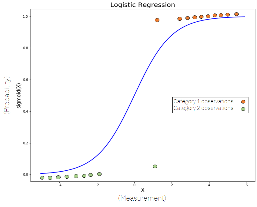
1-dim logistic regression.
We can also think of this as a single-layer ANN with a SIGMOID activation function.
Pos/Cons:
- Simplicity.
- Susceptible to outliers.
- Negatively affected by high correlations in predictors.
- Limited to linear boundaries.
- Generalized and easily outperformed by ANNs.
Characteristics: discriminative
Linear Regression
Solves: Regression
Method: Let \(X \in \mathbb{R}^{D \times n}\) be a matrix where we arranged the n point of our dataset column-wise and \(Y \in \mathbb{R}^{d \times n}\) the values we want to linearly map.
We look for the matrix \(W \in \mathbb{R}^{d \times D}\) such that:
\begin{equation} Y = W X \end{equation}
You can add a bias term by letting the first column of $X$ be made of $1$’s.
This leaves us with an overdetermined system of equations whose solution can be approximated using the least squares method (which minimizes the mean squared error loss):
\begin{equation} W = Y X^T (X X^T)^{-1} \end{equation}
Schematically:
\begin{equation} \vec{x} \rightarrow \text{Linear function} \space \space W \cdot \vec{x} \rightarrow \vec{y} \end{equation}
Pos/Cons:
- Works well with small datasets.
- Linear.
-
- Inverse of a matrix is expensive: \(O(n^a)\) with \(a > 2.3\)
- Susceptible to outliers and high correlations in predictors.
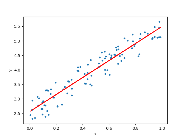
1-dim linear regression.
Characteristics: discriminative
Unsupervised Learning
Notice any discriminative model can become generative if you are willing to assume some prior distribution over the input.
Clustering
Hierarchical clustering
Method: Start by considering each point of your dataset a cluster. Iteratively merge the closest cluster until you have as many clusters as you want.
Pos/Cons:
- Simple
- Number of clusters need to be pre-set
- Isotropic: Only works for spherical clusters
- Optimal not guaranteed
- Slow
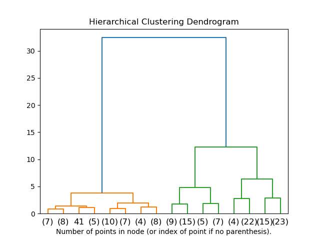
Hierarchical clustering idea.
k-means
Method: Randomly place \(k\) centroids and iteratively repeat these two steps until convergence:
- Assign each point of the dataset to the closest centroid.
- Move the centroid to the center of mass of its assigned points.
Pos/Cons:
- Simple
- Number of clusters need to be pre-set
- Isotropic: Only works for spherical clusters
- Optimal not guaranteed
k-means visualized.
Expectation Maximization
See our post on EM and VI
Spectral clustering
Method: The algorithm consists of two steps:
- Lower dimensionality of the data (using the spectral decomposition of the similarity matrix)
- Perform any simple clustering method (e.g. hierarchical or k-means) in the embedded space.
Dimensionality Reduction
See our posts on dimensionality reduction basics and dimensionality reduction algorithms.
Generative models
See our post on generative models